Understanding the Concept of Value at Risk
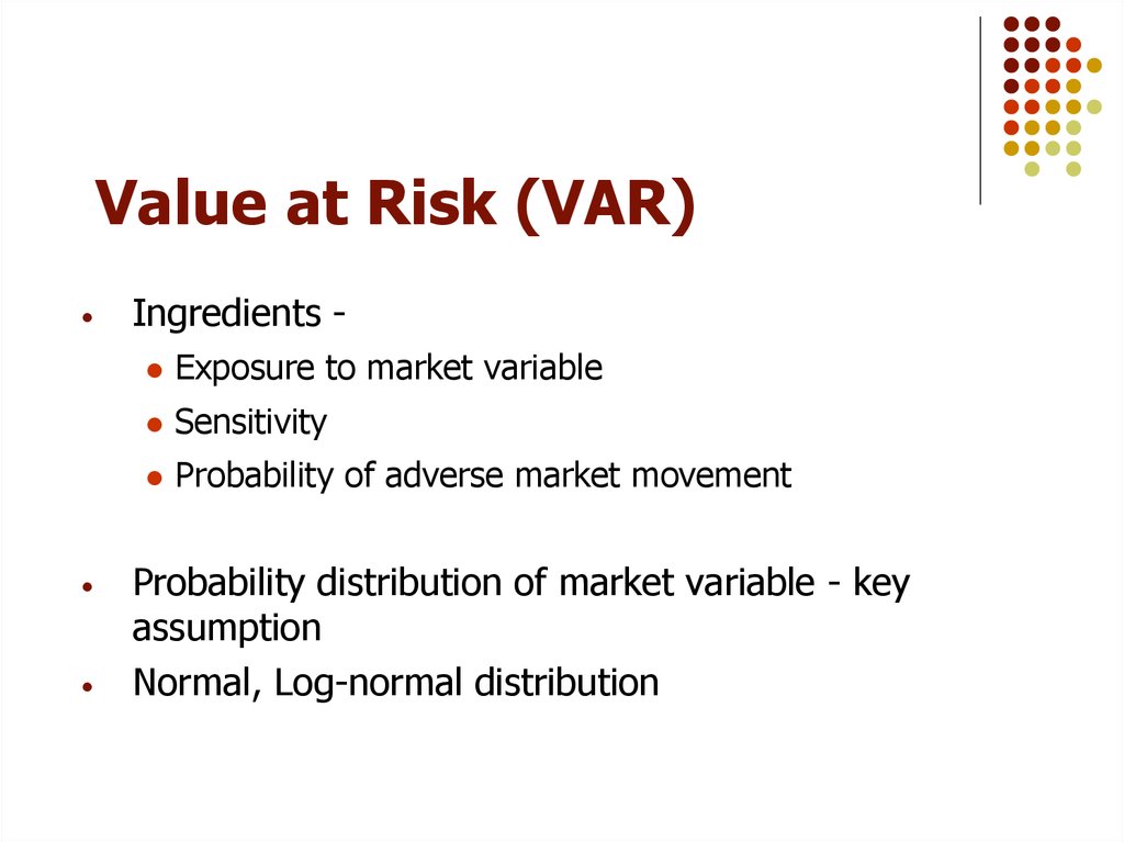
Value at Risk (VaR) is a crucial metric in risk management, enabling financial institutions and investors to quantify potential losses. It estimates the potential loss of a portfolio over a specific time horizon with a given probability. By calculating VaR, investors can better understand the potential downside of their investments, making informed decisions to mitigate risk. In essence, VaR helps investors answer critical questions, such as “What is the potential loss of my portfolio over the next 24 hours?” or “What is the likelihood of my investment losing 10% of its value in the next month?” The concept of VaR is closely tied to the normal distribution, which is a fundamental assumption in many financial models. As we delve into the world of VaR, it’s essential to understand the significance of normal distribution in VaR calculation, which will be discussed in the next section.

Click Image to Find Quantum Products
The Role of Normal Distribution in VaR Calculation
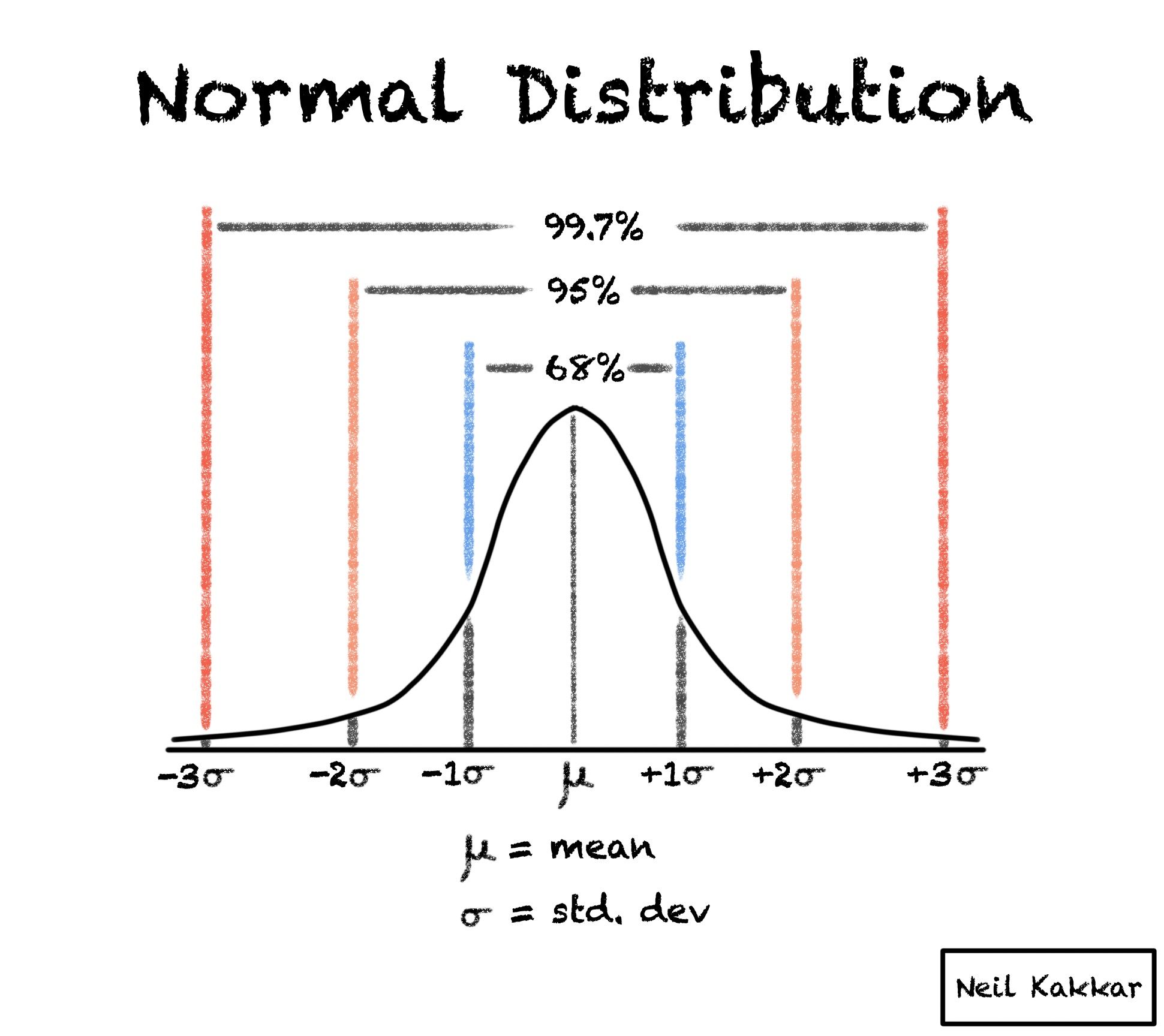
In the calculation of Value at Risk (VaR), normal distribution plays a vital role. The normal distribution, also known as the Gaussian distribution or bell curve, is a statistical concept that assumes that data points are evenly distributed around the mean. In the context of VaR, normal distribution is used to model potential losses, providing a framework for estimating the probability of different outcomes. The normal distribution assumption is crucial in VaR calculation, as it enables the estimation of potential losses with a given confidence level. However, it’s essential to understand the limitations of normal distribution in VaR calculation, including the assumption of normality and the impact of fat tails. Despite these limitations, normal distribution remains a fundamental component of VaR calculation, providing a robust framework for risk management.
How to Calculate VaR Using Normal Distribution
To calculate Value at Risk (VaR) using normal distribution, follow these steps:
Step 1: Determine the confidence level, typically set at 95% or 99%, which represents the probability of not exceeding the VaR threshold.
Step 2: Define the time horizon, which is the period over which the potential loss is calculated, usually expressed in days or weeks.
Step 3: Calculate the standard deviation of the portfolio returns, which represents the volatility of the portfolio.
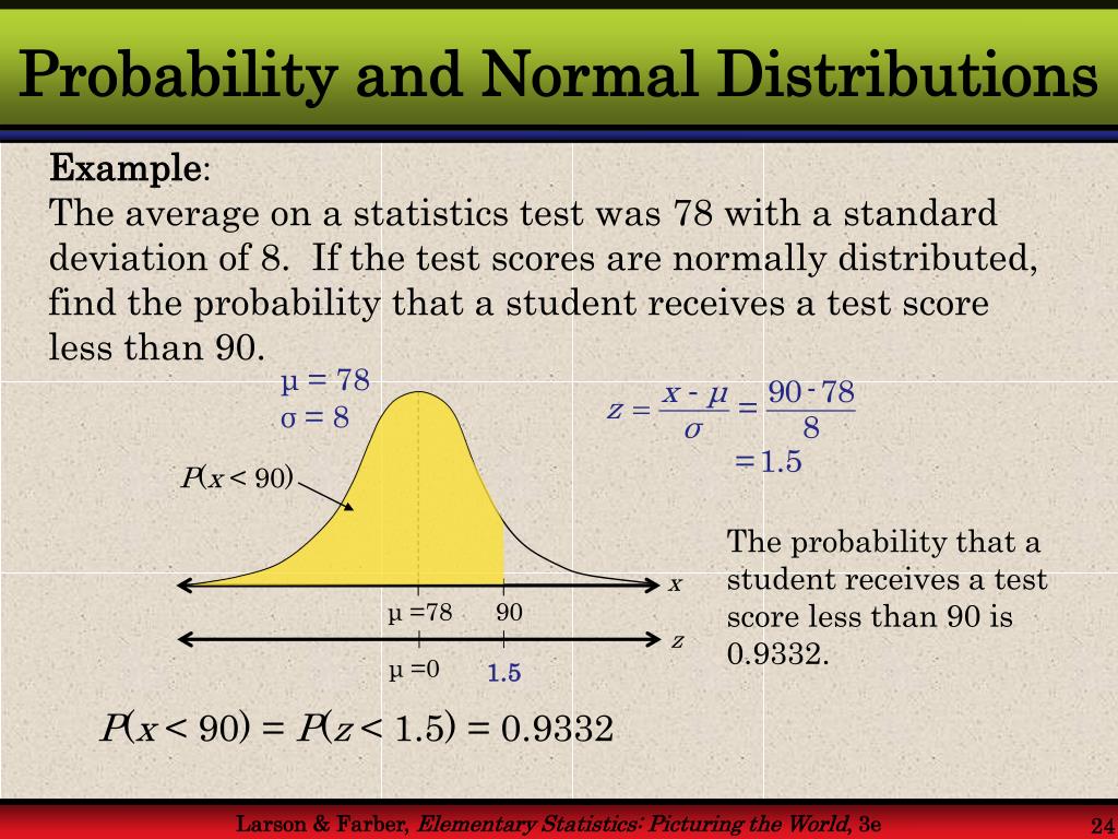
Step 4: Apply the VaR formula: VaR = Z \* σ \* √t, where Z is the Z-score corresponding to the confidence level, σ is the standard deviation, and t is the time horizon.
For example, suppose we want to calculate the 1-day 95% VaR of a portfolio with a standard deviation of 2%. Using a Z-score of 1.645, the VaR would be: VaR = 1.645 \* 2% \* √1 = 3.29%.
In this example, the VaR indicates that there is a 5% probability that the portfolio will lose more than 3.29% of its value over the next day. By understanding the normal distribution value at risk, investors can better quantify and manage their potential losses.
:max_bytes(150000):strip_icc()/dotdash_final_Optimize_Your_Portfolio_Using_Normal_Distribution_Jan_2021-04-a92fef9458844ea0889ea7db57bc0adb.jpg)
Interpreting VaR Results: What Do the Numbers Mean?
Once the Value at Risk (VaR) is calculated, it’s essential to understand the meaning of the results and how to use them to make informed investment decisions. VaR values represent the potential loss of a portfolio over a specific time horizon with a given confidence level. For instance, a 1-day 95% VaR of 3% indicates that there is a 5% probability that the portfolio will lose more than 3% of its value over the next day.
To interpret VaR results effectively, it’s crucial to consider the following factors:
– Confidence level: A higher confidence level (e.g., 99%) indicates a lower probability of exceeding the VaR threshold, while a lower confidence level (e.g., 95%) indicates a higher probability.
– Time horizon: A longer time horizon increases the potential loss, as there is more time for adverse market movements to occur.
– Portfolio composition: VaR results can be influenced by the composition of the portfolio, including the types of assets, their weights, and correlations.
– Market conditions: VaR results can be affected by market conditions, such as volatility, liquidity, and macroeconomic factors.
By understanding the VaR results, investors and financial institutions can make informed decisions about risk management, asset allocation, and capital requirements. For example, a high VaR value may indicate the need to reduce risk exposure, diversify the portfolio, or increase capital buffers. Conversely, a low VaR value may suggest opportunities to take on more risk or optimize portfolio performance.
In the context of normal distribution value at risk, it’s essential to recognize that VaR results are based on historical data and may not accurately capture extreme events or fat-tailed distributions. Therefore, it’s crucial to complement VaR analysis with other risk metrics and stress testing to ensure a comprehensive understanding of potential losses.
Limitations of Normal Distribution in VaR Calculation
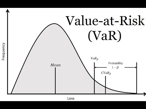
The normal distribution is a widely used assumption in Value at Risk (VaR) calculation, but it has several limitations that can lead to inaccurate results. One of the main limitations is the assumption of normality, which may not always hold true in real-world financial markets. Financial returns often exhibit fat-tailed distributions, which can result in extreme events that are not captured by the normal distribution.
The impact of fat tails on VaR calculation can be significant. Fat-tailed distributions have a higher probability of extreme events, which can lead to larger potential losses than predicted by the normal distribution. This means that VaR values calculated using the normal distribution may underestimate the true risk of a portfolio.
Another limitation of the normal distribution is its inability to capture correlations between different assets in a portfolio. In reality, assets are often correlated, and ignoring these correlations can lead to inaccurate VaR results.
To address these limitations, alternative approaches to VaR calculation have been developed. One such approach is the use of historical simulation, which involves estimating VaR by simulating potential losses based on historical data. This approach can capture fat-tailed distributions and correlations between assets, providing a more accurate estimate of VaR.
Another approach is the use of Monte Carlo simulations, which involve generating random scenarios to estimate potential losses. This approach can also capture fat-tailed distributions and correlations, and can be used to estimate VaR for complex portfolios.
In the context of normal distribution value at risk, it’s essential to recognize the limitations of the normal distribution and consider alternative approaches to VaR calculation. By using a combination of approaches, financial institutions and investors can obtain a more comprehensive understanding of potential losses and make informed decisions about risk management.
Real-World Applications of VaR in Finance
Value at Risk (VaR) is a widely used risk management tool in the financial industry, and its applications are diverse and far-reaching. In this section, we’ll explore how VaR is used in real-world finance, including risk management in banks, investment firms, and hedge funds.
In banks, VaR is used to quantify potential losses and manage risk exposure. For example, a bank may use VaR to determine the potential loss of a loan portfolio over a specific time horizon, such as a day or a week. This information can help the bank to set aside sufficient capital to cover potential losses and maintain regulatory compliance.
In investment firms, VaR is used to manage risk and optimize portfolio performance. For instance, an investment firm may use VaR to determine the potential loss of a portfolio of stocks or bonds over a specific time horizon. This information can help the firm to adjust its portfolio composition and risk exposure to achieve its investment objectives.
In hedge funds, VaR is used to manage risk and maximize returns. Hedge funds often use complex trading strategies and leverage to generate returns, and VaR helps them to quantify and manage the associated risks. By using VaR, hedge funds can identify potential areas of risk and adjust their strategies to minimize losses and maximize returns.
In addition to these examples, VaR is also used in other areas of finance, such as asset management, insurance, and regulatory capital requirements. The widespread adoption of VaR is a testament to its effectiveness in managing risk and quantifying potential losses.
In the context of normal distribution value at risk, it’s essential to recognize the importance of VaR in real-world finance. By understanding how VaR is used in practice, financial institutions and investors can better appreciate its role in managing risk and achieving investment objectives.
Common Mistakes to Avoid in VaR Calculation
When calculating Value at Risk (VaR) using normal distribution, it’s essential to avoid common mistakes that can lead to inaccurate results. In this section, we’ll identify common mistakes to avoid in VaR calculation, including incorrect confidence levels, inadequate data, and ignoring correlations.
One common mistake is using an incorrect confidence level. The confidence level determines the probability of exceeding the VaR threshold, and using an incorrect level can lead to inaccurate results. For example, using a 95% confidence level instead of a 99% confidence level can result in a significantly lower VaR value, which may not accurately reflect the true risk of the portfolio.
Another common mistake is using inadequate data. VaR calculation requires a sufficient amount of high-quality data to produce accurate results. Using inadequate data can lead to inaccurate VaR values, which can result in poor investment decisions. It’s essential to ensure that the data used is relevant, reliable, and sufficient to capture the underlying risks of the portfolio.
Ignoring correlations is another common mistake to avoid. Correlations between different assets in a portfolio can have a significant impact on VaR values. Ignoring these correlations can lead to inaccurate VaR values, which can result in poor investment decisions. It’s essential to account for correlations between assets when calculating VaR using normal distribution.
In the context of normal distribution value at risk, it’s crucial to avoid these common mistakes to ensure accurate results. By understanding the common mistakes to avoid, financial institutions and investors can ensure that their VaR calculations are accurate and reliable, which can help them to make informed investment decisions and manage risk effectively.
Additionally, other common mistakes to avoid include using an incorrect time horizon, ignoring non-normality, and failing to update the VaR model regularly. By avoiding these mistakes, financial institutions and investors can ensure that their VaR calculations are accurate and reliable, which can help them to achieve their investment objectives and manage risk effectively.
Best Practices for Implementing VaR in Your Organization
Implementing Value at Risk (VaR) in an organization requires careful planning, execution, and ongoing monitoring. In this section, we’ll offer best practices for implementing VaR in an organization, including data management, model validation, and ongoing monitoring.
Data management is a critical component of VaR implementation. It’s essential to ensure that the data used for VaR calculation is accurate, complete, and relevant. This includes collecting and storing data on market prices, volatilities, and correlations, as well as ensuring that the data is updated regularly. A robust data management system can help to ensure that VaR calculations are accurate and reliable.
Model validation is another critical component of VaR implementation. It’s essential to validate the VaR model to ensure that it accurately captures the underlying risks of the portfolio. This includes backtesting the model using historical data, as well as stress testing the model to ensure that it can withstand extreme market conditions. A validated VaR model can help to ensure that the organization is adequately prepared for potential losses.
Ongoing monitoring is also essential for effective VaR implementation. It’s essential to regularly review and update the VaR model to ensure that it remains accurate and relevant. This includes monitoring changes in market conditions, as well as updating the model to reflect changes in the portfolio. Ongoing monitoring can help to ensure that the organization remains aware of potential risks and can take proactive steps to manage them.
In the context of normal distribution value at risk, it’s essential to implement VaR in a way that is tailored to the organization’s specific needs and goals. By following best practices for implementing VaR, organizations can ensure that they are adequately prepared for potential losses and can make informed investment decisions.
Additional best practices for implementing VaR include establishing a clear risk management framework, defining risk tolerance and appetite, and ensuring that VaR results are communicated effectively to stakeholders. By following these best practices, organizations can ensure that VaR is integrated into their overall risk management strategy and is used to inform investment decisions.
