What are Markov Decision Processes?
Markov decision processes (MDPs) are a mathematical framework employed for modeling decision-making situations where outcomes are partly random and partly under the control of a decision-maker. MDPs provide a rigorous and systematic approach to decision-making, enabling the optimization of long-term outcomes by balancing immediate rewards and future consequences. The Markov decision processes framework has proven invaluable in various fields, including artificial intelligence, operations research, control theory, and economics.

Click Image to Find Quantum Products

Key Components of Markov Decision Processes
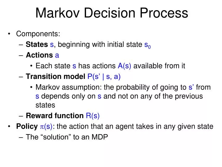
Markov decision processes (MDPs) consist of several fundamental components that interact to form a decision-making model. These elements include states, actions, transition probabilities, and rewards. By understanding these components, one can effectively model and solve decision-making problems using the MDP framework.
- States: A state represents the current situation in which a decision must be made. In MDPs, states are often described using a set of variables that capture relevant information about the environment. For example, in a robot navigation problem, the state might include the robot’s current position, orientation, and the locations of obstacles.
- Actions: Actions are the choices available to the decision-maker within a given state. Actions can be discrete or continuous, depending on the problem. For instance, in the robot navigation example, possible actions might include moving forward, turning left, or turning right.
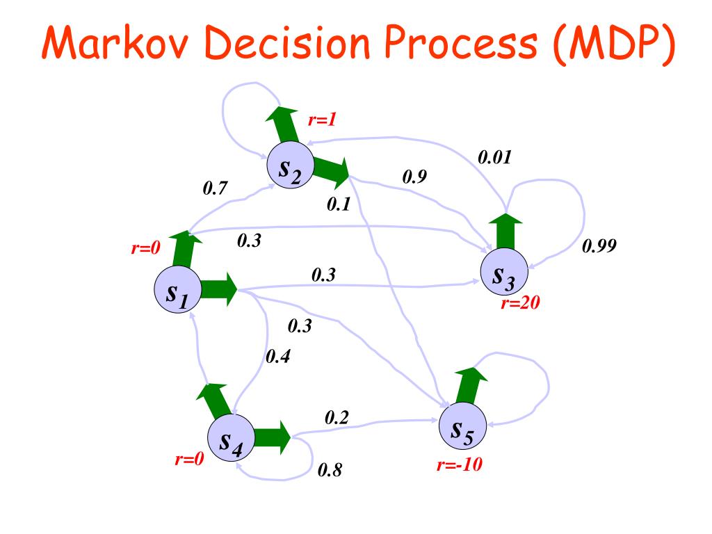
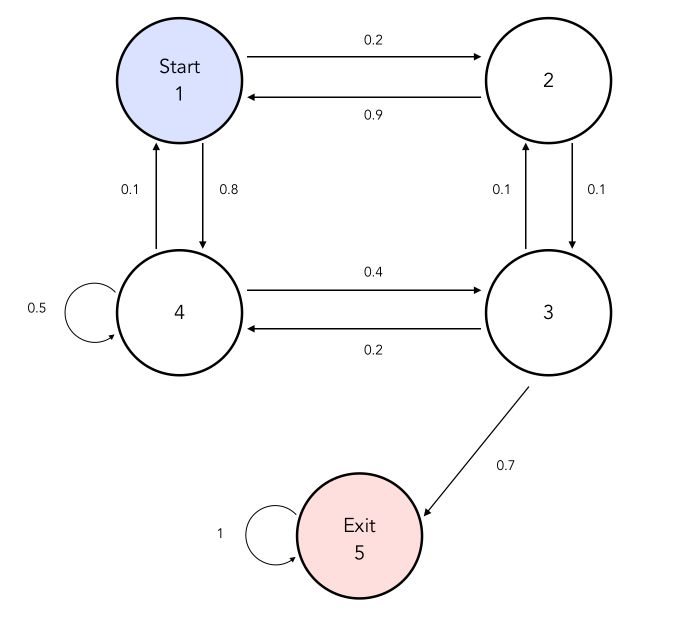
- Transition Probabilities: Transition probabilities describe the likelihood of transitioning from one state to another after taking a specific action. These probabilities capture the randomness inherent in many decision-making scenarios. In the robot navigation example, the transition probabilities might account for the possibility of the robot slipping or deviating from its intended path due to uneven terrain or other factors.
- Rewards: Rewards represent the immediate benefit or cost associated with transitioning from one state to another. Rewards can be positive, negative, or zero, depending on the problem. In the robot navigation example, the reward function might encourage the robot to reach its destination quickly while avoiding obstacles and minimizing energy consumption.
MDPs can be applied to a wide range of real-world problems, such as manufacturing optimization, resource allocation, and autonomous systems control. By accurately modeling the states, actions, transition probabilities, and rewards, decision-makers can leverage the MDP framework to make informed decisions that maximize long-term rewards and improve overall system performance.
The Markov Property and its Role in MDPs
A crucial aspect of Markov decision processes (MDPs) is the Markov property, which simplifies the decision-making process by allowing the future to depend only on the present state, rather than the entire history of past states. This memoryless property significantly reduces the complexity of MDPs, making them more manageable for analysis and optimization.
Definition of the Markov Property
In the context of MDPs, the Markov property states that the probability of transitioning to the next state depends only on the current state and action, and not on the sequence of previous states and actions. Mathematically, this can be expressed as:
P(S’|S, A) = P(S’|H)
where S’ is the next state, S is the current state, A is the action taken in the current state, and H is the history of past states and actions. The Markov property holds if and only if the above equation is true.
Implications of the Markov Property
The Markov property has several important implications for MDPs. First, it allows for the decomposition of the value function, which represents the expected total reward of following a policy from a given state, into a sum of expected rewards over individual time steps. This decomposition, in turn, enables the use of dynamic programming techniques for solving MDPs, as discussed in a later section.
Second, the Markov property enables the use of probability theory to model and analyze MDPs. By focusing on the transition probabilities between states, rather than the entire history of past states, the analysis of MDPs becomes more tractable and intuitive. This simplification is particularly valuable when dealing with complex decision-making scenarios, where the number of possible histories can grow exponentially with the number of time steps.
Example of the Markov Property
Consider a simple weather model where the state space consists of two states: sunny and rainy. The weather on each day is assumed to be a Markov decision process, meaning that the probability of rain or sunshine on a given day depends only on the weather of the previous day and not on the entire history of past weather conditions. In this case, the Markov property holds, and the weather model can be analyzed using MDP techniques.
How to Formulate a Problem as a Markov Decision Process
Formulating a decision-making problem as a Markov decision process (MDP) involves several steps, which can be broken down as follows:
- Define the state space: Identify the set of all possible states that the system can be in. Each state should capture all relevant information about the system’s current situation. For example, in a robot navigation problem, the state space might include the robot’s position, orientation, and the locations of obstacles.
- Define the action space: Identify the set of all possible actions that can be taken in each state. Actions should be chosen such that they can affect the system’s transition between states. For instance, in the robot navigation example, possible actions might include moving forward, turning left, or turning right.
- Define the transition probabilities: Specify the probability of transitioning from one state to another given a particular action. Transition probabilities should capture the randomness inherent in many decision-making scenarios. In the robot navigation example, the transition probabilities might account for the possibility of the robot slipping or deviating from its intended path due to uneven terrain or other factors.
- Define the reward function: Assign a reward or cost to each transition between states. Rewards should reflect the desirability of the outcome associated with that transition. In the robot navigation example, the reward function might encourage the robot to reach its destination quickly while avoiding obstacles and minimizing energy consumption.
Once a problem has been formulated as an MDP, various algorithms can be employed to solve it, as discussed in subsequent sections. It is important to note that the formulation process may require some trial and error, as different state, action, and reward definitions can lead to significantly different outcomes. Careful consideration should be given to the choice of state and action spaces, as well as the design of the reward function, to ensure that the MDP accurately reflects the decision-making problem at hand.
Solving Markov Decision Processes: Dynamic Programming
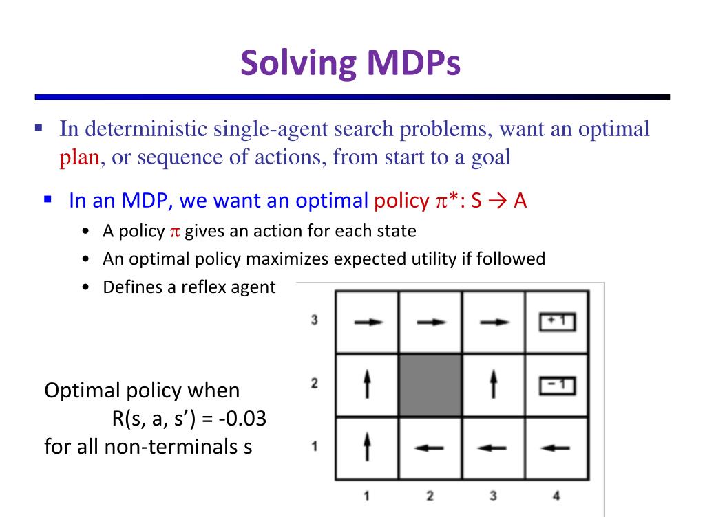
Dynamic programming is a powerful method for solving Markov decision processes (MDPs) that leverages the Bellman optimality principle to recursively decompose the value function into smaller, more manageable components. The Bellman optimality principle states that the optimal value function can be expressed as a function of the optimal value function at the next time step, discounted by the discount factor. Mathematically, this can be represented as:
V*(s) = maxa ∑s’ P(s’, r|s, a) [r + γV*(s’)]
where V*(s) is the optimal value function for state s, a is an action, P(s’, r|s, a) is the probability of transitioning to state s’ and receiving reward r when taking action a in state s, and γ is the discount factor.
Dynamic programming algorithms
Alternative Approaches to Solving MDPs
While dynamic programming is a powerful method for solving Markov decision processes (MDPs), it is not the only approach available. Several alternative methods have been developed, each with its advantages and disadvantages. In this section, we will discuss three such methods: Monte Carlo methods, temporal difference learning, and reinforcement learning.
Monte Carlo Methods
Monte Carlo methods are a class of simulation-based techniques that use random sampling to estimate the value function of an MDP. These methods are particularly useful when the transition probabilities are unknown or difficult to estimate. Monte Carlo methods can be further divided into two categories: every-visit and first-visit methods. Every-visit methods estimate the average reward over all visits to a state, while first-visit methods estimate the reward obtained on the first visit to a state.
Temporal Difference Learning
Temporal difference learning (TD learning) is a family of methods that combine elements of both Monte Carlo methods and dynamic programming. TD learning updates the value function based on the difference between the estimated value of the current state and the estimated value of the next state, without waiting for the entire episode to complete. TD learning can be particularly useful in situations where the number of time steps is large or infinite, as it does not require explicit knowledge of the transition probabilities.
Reinforcement Learning
Reinforcement learning (RL) is a general framework for learning optimal policies in MDPs through trial and error. RL algorithms typically operate by interacting with an environment, receiving rewards or penalties based on their actions, and updating their policies accordingly. RL can be particularly useful in situations where the transition probabilities are unknown or difficult to estimate, as it does not require explicit knowledge of these probabilities.
Each of these alternative approaches has its advantages and disadvantages. Monte Carlo methods are well-suited for situations where the transition probabilities are unknown or difficult to estimate, but they can be computationally expensive and may require a large number of simulations to achieve accurate estimates. TD learning can be more efficient than Monte Carlo methods, as it updates the value function incrementally, but it may be less stable in some situations. Reinforcement learning can be particularly useful in complex environments with many states and actions, but it can be challenging to design RL algorithms that converge to optimal policies in a reasonable amount of time.
In practice, the choice of method depends on the specific problem at hand, as well as factors such as computational resources, the availability of data, and the desired level of accuracy. By understanding the strengths and limitations of each approach, decision-makers can make informed choices about which method to use in a given situation.
Advanced Topics in Markov Decision Processes
Markov decision processes (MDPs) provide a powerful framework for modeling decision-making problems in a wide range of applications. However, there are several advanced topics in MDPs that require special consideration. In this section, we will explore three such topics: continuous state spaces, partial observability, and multi-agent systems.
Continuous State Spaces
In many real-world applications, the state space of an MDP is continuous rather than discrete. For example, in a robotic arm manipulation task, the state space might include the position and velocity of each joint, which can take on an infinite number of values. Continuous state spaces present unique challenges, as many of the standard algorithms for solving MDPs, such as value iteration and policy iteration, are designed for discrete state spaces. Several methods have been developed for addressing continuous state spaces, including function approximation, discretization, and numerical methods such as finite difference and Galerkin methods.
Partial Observability
In many decision-making problems, the decision-maker does not have complete information about the current state of the system. Instead, the decision-maker may only have access to partial observations, which provide limited information about the state. Partially observable Markov decision processes (POMDPs) extend the standard MDP framework to handle partial observability. In a POMDP, the decision-maker maintains a belief state, which represents the probability distribution over the possible states of the system. The belief state is updated based on the observed outcomes and the transition probabilities of the system. Solving POMDPs is generally more challenging than solving standard MDPs, as the belief state can be high-dimensional and complex to compute.
Multi-Agent Systems
Many real-world decision-making problems involve multiple agents interacting with each other. For example, in a traffic control system, there may be multiple intersections, each controlled by a separate agent. Multi-agent Markov decision processes (MMDPs) extend the standard MDP framework to handle multiple agents. In an MMDP, each agent has its own action space and reward function, and the transition probabilities depend on the joint actions of all agents. Solving MMDPs is generally more challenging than solving standard MDPs, as the joint action space can be large and complex, and the agents may have conflicting objectives.
Each of these advanced topics presents unique challenges and opportunities for researchers and practitioners working with MDPs. By understanding the complexities and potential solutions associated with these topics, decision-makers can apply MDPs to a wider range of problems and achieve more accurate and effective decision-making.

Practical Considerations and Applications of Markov Decision Processes
Markov decision processes (MDPs) have been successfully applied to a wide range of decision-making problems in various industries. However, there are several practical considerations that must be taken into account when implementing MDPs in real-world scenarios. In this section, we will discuss three such considerations: computational complexity, numerical stability, and real-world constraints.
Computational Complexity
Solving MDPs can be computationally intensive, particularly for large-scale problems with many states and actions. The computational complexity of solving an MDP depends on several factors, including the size of the state and action spaces, the sparsity of the transition probabilities, and the desired level of accuracy. Several methods have been developed for reducing the computational complexity of solving MDPs, including approximation algorithms, heuristic search algorithms, and parallel computing techniques.
Numerical Stability
Numerical stability is an important consideration when implementing MDPs, particularly when using numerical methods such as value iteration and policy iteration. Numerical instability can arise due to several factors, including rounding errors, truncation errors, and approximation errors. Several methods have been developed for improving the numerical stability of MDP algorithms, including regularization techniques, stability-enhancing transformations, and convergence acceleration techniques.
Real-World Constraints
Real-world decision-making problems often involve complex constraints that must be taken into account when formulating and solving MDPs. Examples of such constraints include physical constraints (e.g., limits on the range of motion of a robotic arm), temporal constraints (e.g., deadlines for completing a task), and resource constraints (e.g., budget limitations). Several methods have been developed for incorporating constraints into MDPs, including constraint programming techniques, linear programming techniques, and integer programming techniques.
By taking these practical considerations into account, decision-makers can effectively apply MDPs to a wide range of real-world problems in various industries, such as robotics, finance, and healthcare. For example, in robotics, MDPs have been used for motion planning, manipulation planning, and autonomous navigation. In finance, MDPs have been used for portfolio optimization, risk management, and option pricing. In healthcare, MDPs have been used for treatment planning, resource allocation, and disease modeling.
In conclusion, Markov decision processes provide a powerful framework for modeling and solving decision-making problems in a wide range of applications. By understanding the key components of MDPs, the Markov property, and the steps required to formulate a problem as an MDP, decision-makers can effectively apply MDPs to real-world problems. Furthermore, by taking into account practical considerations such as computational complexity, numerical stability, and real-world constraints, decision-makers can ensure that their MDP models are accurate, efficient, and effective.