How to Calculate a Sharpe Ratio

What is the Sharpe Ratio and Why Does it Matter?

In the realm of investment analysis, the Sharpe Ratio is a widely recognized metric for evaluating investment performance. It provides a risk-adjusted measure of return, helping investors make informed decisions about their portfolios. But what exactly is the Sharpe Ratio, and why is it so crucial in investment analysis? The Sharpe Ratio is a powerful tool for understanding the relationship between risk and return, allowing investors to compare different investments and make more informed decisions. As investors seek to maximize returns while minimizing risk, understanding how to calculate a Sharpe Ratio is essential for making informed investment decisions. In this article, we’ll delve into the world of risk-adjusted returns, exploring the importance of the Sharpe Ratio and how to calculate it.

Breaking Down the Sharpe Ratio Formula

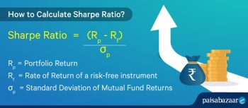
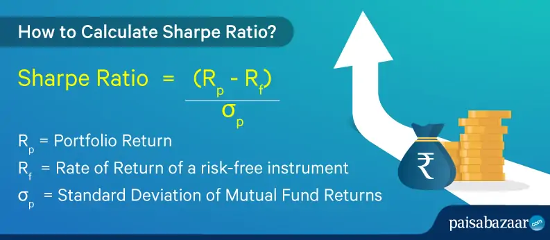
The Sharpe Ratio formula is a straightforward yet powerful tool for evaluating investment performance. To calculate the Sharpe Ratio, investors need to understand the three key components: expected return, standard deviation, and risk-free rate. The formula is as follows: Sharpe Ratio = (Expected Return – Risk-Free Rate) / Standard Deviation. Let’s break down each component to understand how to calculate a Sharpe Ratio:

The expected return represents the anticipated return of an investment, typically expressed as a percentage. The risk-free rate is the return of a risk-free asset, such as a U.S. Treasury bond. The standard deviation measures the volatility of an investment, providing a sense of the investment’s risk profile. By combining these three components, the Sharpe Ratio provides a risk-adjusted measure of return, allowing investors to compare different investments and make more informed decisions.

In the next section, we’ll walk through a step-by-step example of calculating the Sharpe Ratio, using real-world data to illustrate the process.

Understanding the Sharpe Ratio Calculation: A Step-by-Step Example

To illustrate how to calculate a Sharpe Ratio, let’s consider a hypothetical investment scenario. Suppose we want to evaluate the performance of a stock portfolio with an expected return of 12% per annum, a standard deviation of 15%, and a risk-free rate of 4% per annum. We’ll walk through the calculation process step-by-step:

Step 1: Calculate the excess return by subtracting the risk-free rate from the expected return: Excess Return = 12% – 4% = 8%

Step 2: Calculate the standard deviation of the portfolio: Standard Deviation = 15%

Step 3: Calculate the Sharpe Ratio by dividing the excess return by the standard deviation: Sharpe Ratio = 8% / 15% = 0.53

In this example, the Sharpe Ratio is 0.53, indicating that for every unit of risk taken, the portfolio generates a return of 0.53. A higher Sharpe Ratio indicates better risk-adjusted performance. However, it’s essential to consider the limitations of the Sharpe Ratio, such as its sensitivity to volatility and assumptions about normal distributions, which we’ll discuss in the next section.

By following these steps, investors can calculate the Sharpe Ratio for their investments and gain a deeper understanding of their risk-adjusted returns. In the next section, we’ll explore how to interpret the results of the Sharpe Ratio calculation and what they mean for investment decisions.

Interpreting Sharpe Ratio Results: What Do the Numbers Mean?

Once the Sharpe Ratio is calculated, investors need to understand what the results mean in the context of their investment decisions. A Sharpe Ratio of 1 or higher is generally considered good, indicating that the investment has generated excess returns relative to its risk. A ratio of 2 or higher is considered excellent, suggesting that the investment has produced outstanding risk-adjusted returns.

On the other hand, a Sharpe Ratio of less than 1 indicates that the investment has not generated sufficient returns to justify its risk. A negative Sharpe Ratio suggests that the investment has performed poorly, and investors may want to reconsider their allocation.

It’s essential to note that the Sharpe Ratio is a relative measure, and its interpretation depends on the investment’s peer group or benchmark. For instance, a Sharpe Ratio of 0.5 may be acceptable for a conservative investment, but it may be considered poor for a more aggressive investment.

When interpreting Sharpe Ratio results, investors should also consider the following factors:

• The investment’s time horizon: A longer time horizon may justify a lower Sharpe Ratio, as the investment has more time to recover from potential losses.
• The investment’s risk profile: A higher-risk investment may require a higher Sharpe Ratio to justify its risk.
• The market environment: A Sharpe Ratio calculated during a bull market may not be comparable to one calculated during a bear market.

By understanding how to interpret the Sharpe Ratio results, investors can make more informed decisions about their investments and optimize their portfolios for better risk-adjusted returns.

Common Challenges and Limitations of the Sharpe Ratio

The Sharpe Ratio is a widely used metric, but it’s not without its limitations. One of the primary challenges is its sensitivity to volatility. The Sharpe Ratio assumes that returns are normally distributed, which may not always be the case. In reality, returns can be skewed or exhibit fat tails, leading to inaccurate risk assessments.

Another limitation is that the Sharpe Ratio only considers historical data, which may not be representative of future performance. This can lead to overfitting or underestimating risk. Furthermore, the Sharpe Ratio does not account for non-normal distributions, such as those with skewness or kurtosis.

To mitigate these limitations, investors can employ several strategies:

• Use alternative risk metrics, such as Value-at-Risk (VaR) or Expected Shortfall (ES), to complement the Sharpe Ratio.
• Apply robustness tests to ensure that the Sharpe Ratio is not overly sensitive to outliers or extreme events.
• Use Monte Carlo simulations or stress testing to estimate potential losses and improve risk assessment.
• Consider using more advanced risk-adjusted return metrics, such as the Sortino Ratio or the Treynor Ratio, which may better capture the nuances of investment risk.

By acknowledging the limitations of the Sharpe Ratio and incorporating these strategies, investors can develop a more comprehensive understanding of risk-adjusted returns and make more informed investment decisions.

Sharpe Ratio vs. Other Risk-Adjusted Return Metrics

While the Sharpe Ratio is a widely used metric, it’s not the only game in town. Other popular risk-adjusted return metrics include the Sortino Ratio and the Treynor Ratio. Each of these metrics has its strengths and weaknesses, and investors should understand the differences to make informed decisions.

The Sortino Ratio is similar to the Sharpe Ratio, but it uses a different measure of risk: downside deviation instead of standard deviation. This makes it more sensitive to extreme losses, which can be beneficial for investors who prioritize capital preservation. The Sortino Ratio is particularly useful for evaluating investments with non-normal distributions or those that exhibit skewness.

The Treynor Ratio, on the other hand, uses a beta-based approach to measure risk. This makes it more suitable for evaluating investments with a high degree of market exposure. The Treynor Ratio is also more sensitive to changes in market conditions, which can be beneficial for investors who need to adapt quickly to shifting market environments.

When deciding which metric to use, investors should consider their investment goals and risk tolerance. The Sharpe Ratio is a good all-around choice, but the Sortino Ratio may be more suitable for conservative investors, while the Treynor Ratio may be more suitable for aggressive investors.

Ultimately, the key is to understand the strengths and weaknesses of each metric and use them in conjunction to gain a more comprehensive understanding of risk-adjusted returns. By doing so, investors can make more informed decisions and optimize their portfolios for better performance.

Practical Applications of the Sharpe Ratio in Investment Analysis

The Sharpe Ratio is a powerful tool in investment analysis, and its applications are diverse and far-reaching. In this section, we’ll explore how the Sharpe Ratio is used in real-world investment analysis, including portfolio optimization, asset allocation, and performance evaluation.

Portfolio Optimization: The Sharpe Ratio is often used to optimize portfolios by identifying the most efficient allocation of assets. By calculating the Sharpe Ratio for different asset combinations, investors can determine the optimal mix of assets that maximizes returns while minimizing risk.

Asset Allocation: The Sharpe Ratio can also be used to evaluate the performance of different asset classes, such as stocks, bonds, and commodities. By comparing the Sharpe Ratios of different asset classes, investors can determine the most attractive investment opportunities and allocate their assets accordingly.

Performance Evaluation: The Sharpe Ratio is a valuable tool for evaluating the performance of investment managers and funds. By calculating the Sharpe Ratio for a particular fund or manager, investors can assess their risk-adjusted returns and make informed decisions about whether to invest or redeem.

In addition to these applications, the Sharpe Ratio can also be used to evaluate the performance of individual securities, such as stocks and bonds. By calculating the Sharpe Ratio for a particular security, investors can assess its risk-adjusted returns and make informed decisions about whether to buy or sell.

Overall, the Sharpe Ratio is a versatile metric that can be applied in a variety of investment contexts. By understanding how to calculate and interpret the Sharpe Ratio, investors can make more informed decisions and achieve their investment goals.

Conclusion: Mastering the Sharpe Ratio for Informed Investment Decisions

In conclusion, the Sharpe Ratio is a powerful tool in investment analysis, providing a comprehensive measure of risk-adjusted returns. By understanding how to calculate and interpret the Sharpe Ratio, investors can make more informed decisions and achieve their investment goals.

Throughout this article, we’ve explored the components of the Sharpe Ratio formula, walked through a step-by-step example of calculating the Sharpe Ratio, and discussed how to interpret the results. We’ve also addressed common challenges and limitations of the Sharpe Ratio, compared it to other risk-adjusted return metrics, and explored its practical applications in investment analysis.

By mastering the Sharpe Ratio, investors can gain a deeper understanding of their investments and make more informed decisions. Whether you’re a seasoned investor or just starting out, understanding how to calculate a Sharpe Ratio can help you navigate the complex world of investment analysis and achieve your financial goals.

Remember, the Sharpe Ratio is just one tool in the investor’s toolkit. By combining it with other metrics and approaches, investors can gain a more complete picture of their investments and make more informed decisions. With practice and patience, investors can unlock the full potential of the Sharpe Ratio and achieve success in the world of investment analysis.