What is Cubic Spline Interpolation and Why is it Important?
In data analysis and visualization, cubic spline interpolation is a powerful technique used to approximate complex data sets. This method is particularly useful when dealing with noisy or incomplete data, as it can effectively fill in gaps and smooth out irregularities. Cubic spline interpolation in MATLAB is a crucial technique for researchers and engineers, offering a high degree of accuracy and flexibility. By applying cubic spline interpolation in MATLAB, users can gain valuable insights into their data, identify patterns, and make informed decisions. The benefits of cubic spline interpolation in MATLAB include its ability to handle large datasets, provide smooth and continuous curves, and offer a high degree of customization. In this article, we will explore the world of cubic spline interpolation in MATLAB, providing a comprehensive guide to its implementation, applications, and benefits.

Click Image to Find Quantum Products

How to Implement Cubic Spline Interpolation in MATLAB
To implement cubic spline interpolation in MATLAB, users can utilize the built-in `spline` function. This function takes in a set of data points and returns a cubic spline interpolant that can be used to estimate values at intermediate points. The basic syntax for the `spline` function is `pp = spline(x, y)`, where `x` and `y` are the input data points. The output `pp` is a piecewise polynomial structure that can be used to evaluate the cubic spline interpolant at any point within the range of the input data. For example, to evaluate the interpolant at a point `x_query`, users can use the command `y_query = ppval(pp, x_query)`. In addition to the basic `spline` function, MATLAB also provides a range of optional parameters and functions that can be used to customize the cubic spline interpolation process. These include the `spline` function with optional parameters, such as `pp = spline(x, y, ‘method’, ‘interp’)`, and the `mkpp` function, which can be used to create a piecewise polynomial structure from a set of data points. By mastering the `spline` function and its associated tools, users can effectively implement cubic spline interpolation in MATLAB and unlock the full potential of this powerful technique.
Understanding the Mathematics Behind Cubic Spline Interpolation
Cubic spline interpolation in MATLAB is built upon a foundation of mathematical concepts, including polynomial equations, knots, and boundary conditions. At its core, cubic spline interpolation involves dividing a dataset into a series of intervals, each of which is approximated by a cubic polynomial. These polynomials are then pieced together to form a smooth, continuous curve that passes through the original data points. The process of creating this curve involves solving a system of linear equations, which can be represented in matrix form. The resulting matrix equation can be solved using a variety of techniques, including Gaussian elimination and LU decomposition. In addition to the polynomial equations, cubic spline interpolation also relies on the concept of knots, which are the points at which the individual polynomials are joined together. The placement and spacing of these knots can have a significant impact on the accuracy and smoothness of the resulting curve. Finally, boundary conditions play a critical role in cubic spline interpolation, as they determine the behavior of the curve at its endpoints. By understanding these underlying mathematical concepts, users can gain a deeper appreciation for the power and flexibility of cubic spline interpolation in MATLAB.

Advantages of Cubic Spline Interpolation Over Other Methods
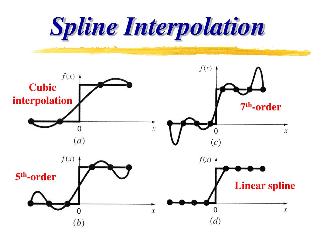
Cubic spline interpolation in MATLAB offers several advantages over other interpolation methods, making it a popular choice for data analysis and visualization. One of the primary benefits of cubic spline interpolation is its ability to produce smooth, continuous curves that accurately capture the underlying trends in the data. This is in contrast to linear interpolation, which can produce jagged, discontinuous curves that fail to capture the nuances of the data. Additionally, cubic spline interpolation is more flexible than polynomial interpolation, as it can be used to model complex, non-linear relationships between variables. Furthermore, cubic spline interpolation is well-suited for handling noisy or irregularly-spaced data, making it a valuable tool for real-world applications. Another advantage of cubic spline interpolation is its ability to be used for both interpolation and extrapolation, allowing users to make predictions about future data points. Overall, the advantages of cubic spline interpolation in MATLAB make it a powerful technique for data analysis and visualization, particularly in fields such as engineering, physics, and computer science.
Real-World Applications of Cubic Spline Interpolation in MATLAB
Cubic spline interpolation in MATLAB has a wide range of practical applications across various fields, including engineering, physics, and computer science. In engineering, cubic spline interpolation is used to model complex systems, such as mechanical systems, electrical circuits, and thermal systems. For instance, it can be used to interpolate temperature data in a thermal system, allowing engineers to predict temperature distributions and optimize system design. In physics, cubic spline interpolation is used to model complex phenomena, such as particle trajectories and electromagnetic fields. For example, it can be used to interpolate particle position data, enabling physicists to study particle behavior and interactions. In computer science, cubic spline interpolation is used in computer-aided design (CAD) and computer-aided engineering (CAE) to create smooth curves and surfaces for design and simulation. Additionally, it is used in data analysis and visualization to create smooth, continuous curves that accurately capture the underlying trends in the data. By using cubic spline interpolation in MATLAB, researchers and practitioners can gain valuable insights into complex systems and phenomena, and make informed decisions based on accurate predictions and simulations.

Common Pitfalls and Troubleshooting in Cubic Spline Interpolation
When implementing cubic spline interpolation in MATLAB, several common pitfalls and issues can arise, leading to inaccurate or misleading results. One common error is incorrect data preparation, such as failing to remove outliers or handle missing values. This can lead to poor interpolation results and inaccurate predictions. Another common issue is selecting the wrong type of cubic spline interpolation, such as using a clamped spline instead of a natural spline. This can result in inaccurate boundary conditions and poor interpolation results. Additionally, users may encounter issues with the `spline` function, such as incorrect syntax or insufficient data points. To troubleshoot these issues, it is essential to carefully review the data and code, and to use visualization tools to inspect the interpolated curves. By being aware of these common pitfalls and taking steps to avoid them, users can ensure accurate and reliable results when using cubic spline interpolation in MATLAB. For example, users can use the `plot` function to visualize the interpolated curve and identify any anomalies or inaccuracies. By using these troubleshooting techniques, users can overcome common issues and achieve accurate and reliable results with cubic spline interpolation in MATLAB.
Visualizing Cubic Spline Interpolation Results in MATLAB
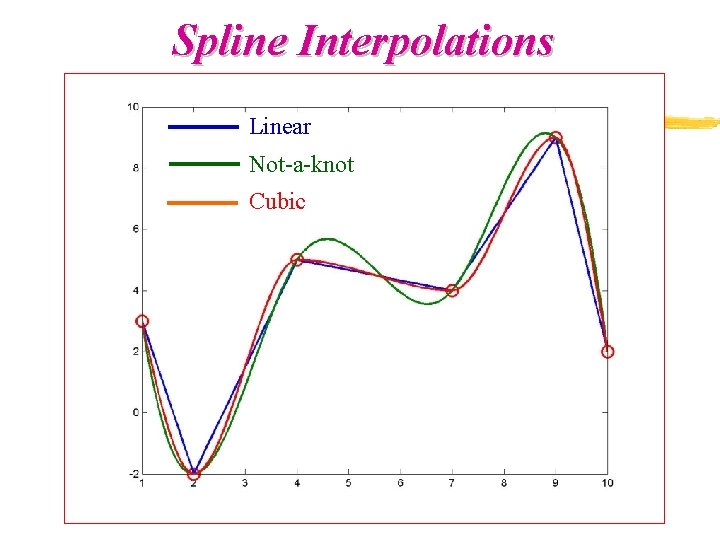
Effective visualization of cubic spline interpolation results is crucial in MATLAB to gain insights into the interpolated curves and make informed decisions. MATLAB provides a range of visualization tools, such as plots and graphs, to illustrate the interpolated curves. To visualize the results of cubic spline interpolation in MATLAB, users can use the `plot` function to create a 2D plot of the interpolated curve. For example, the command `plot(x, y, ‘o’, x, yy, ‘-‘)` can be used to create a plot of the original data points and the interpolated curve. Additionally, users can use the `plot3` function to create a 3D plot of the interpolated surface. By using these visualization tools, users can gain a deeper understanding of the interpolated curves and identify any anomalies or inaccuracies. Furthermore, visualization can help users to compare the results of cubic spline interpolation with other interpolation methods, such as linear and polynomial interpolation. By effectively visualizing the results of cubic spline interpolation in MATLAB, users can unlock the full potential of this powerful technique and make informed decisions in data analysis and visualization. For instance, in engineering, visualization of cubic spline interpolation results can help to identify areas of high stress or strain in a mechanical system, enabling engineers to optimize system design and improve performance.

Best Practices for Cubic Spline Interpolation in MATLAB
When implementing cubic spline interpolation in MATLAB, following best practices is essential to ensure accurate and reliable results. One key best practice is to carefully prepare the data, including removing outliers and handling missing values. This can be achieved using MATLAB’s built-in data manipulation functions, such as `rmoutliers` and `fillmissing`. Another important best practice is to select the appropriate type of cubic spline interpolation, such as clamped or natural spline, depending on the specific problem requirements. Additionally, users should carefully choose the knot points and boundary conditions to ensure a smooth and accurate interpolation. Furthermore, it is essential to validate the results of cubic spline interpolation by comparing them with other interpolation methods and visualizing the interpolated curves. By following these best practices, users can ensure that their implementation of cubic spline interpolation in MATLAB is accurate, reliable, and effective. For example, in engineering, following best practices for cubic spline interpolation can help to improve the accuracy of stress analysis and optimize system design. By incorporating these expert tips and best practices into their workflow, users can unlock the full potential of cubic spline interpolation in MATLAB and achieve superior results in data analysis and visualization.
