Understanding Conditional Probability: The Foundation of Bayes’ Formula
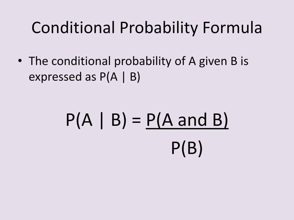
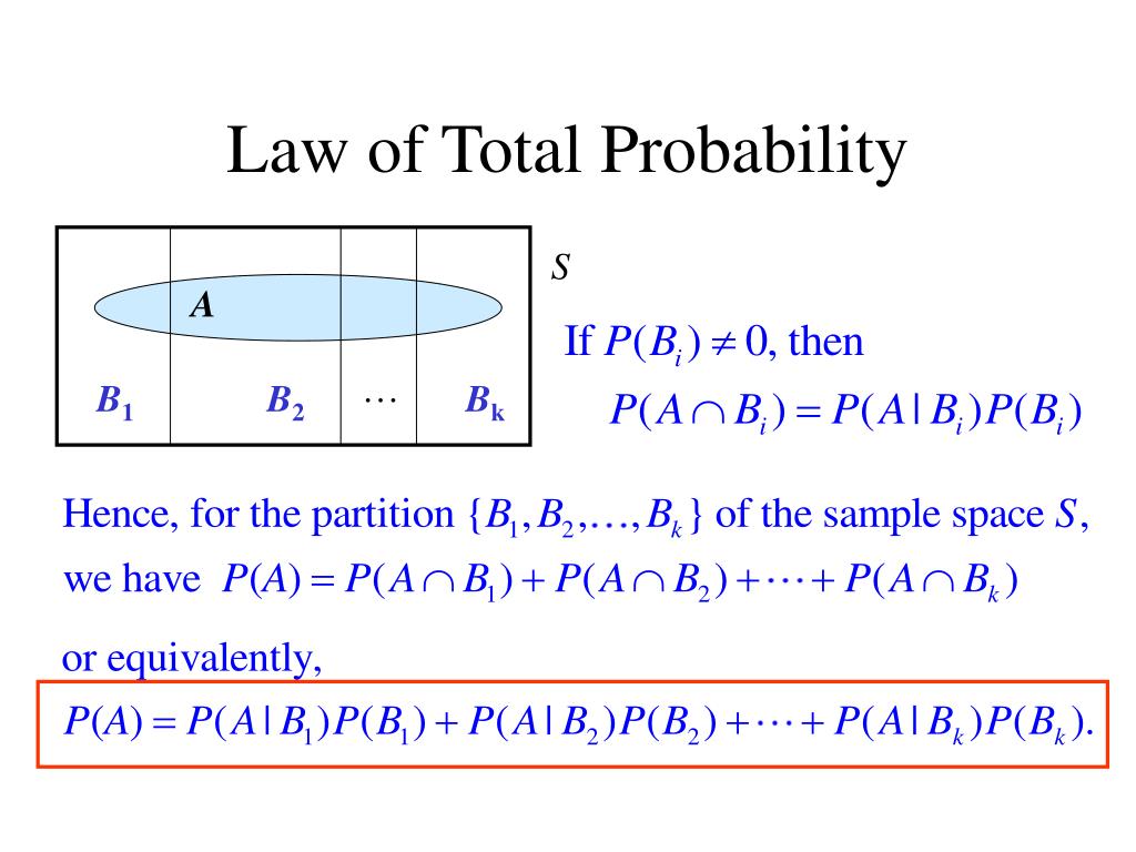
Conditional probability is a fundamental concept in probability theory, playing a crucial role in understanding the likelihood of events occurring. It is essential in real-world applications, such as medicine, finance, and machine learning, where it helps professionals make informed decisions based on data analysis. In essence, conditional probability is the probability of an event occurring given that another event has occurred. This concept forms the basis of Bayes’ formula for conditional probability, a powerful tool for updating probabilities based on new information.
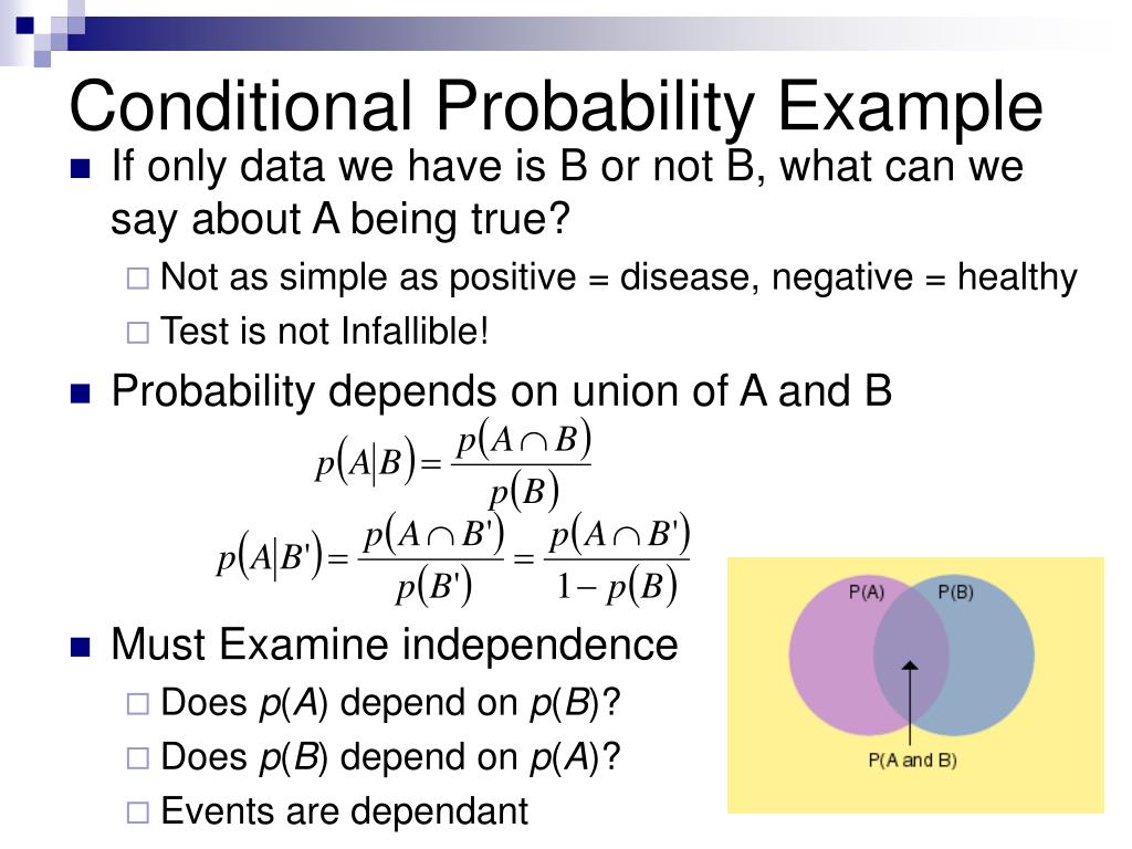
To illustrate the concept, consider a simple example. Suppose we want to determine the probability of a person having a disease given that they have tested positive for it. In this scenario, the probability of the person having the disease is conditional on the test result. This is a classic example of conditional probability, where the occurrence of one event (testing positive) affects the probability of another event (having the disease).
In contrast, joint probability refers to the probability of two or more events occurring simultaneously. For instance, the probability of a person having a disease and testing positive for it is a joint probability. While joint probability is useful in certain contexts, conditional probability provides a more nuanced understanding of the relationships between events.
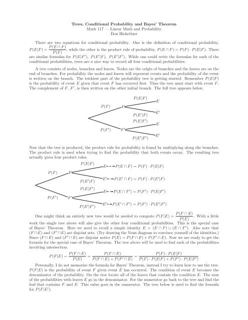
Bayes’ formula for conditional probability is a mathematical expression that updates the probability of an event based on new information. It is a powerful tool for decision-making under uncertainty, and its applications are vast and diverse. By understanding conditional probability, we can unlock the power of Bayes’ formula and make more informed decisions in various fields.
What is Bayes’ Formula? A Mathematical Breakdown
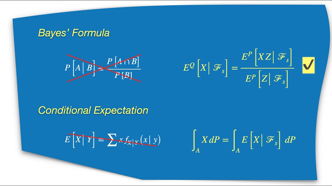
Bayes’ formula is a mathematical expression that describes the probability of an event occurring given that another event has occurred. It is a fundamental concept in probability theory, and its application is crucial in various fields, including medicine, finance, and machine learning. The formula is named after Reverend Thomas Bayes, who first introduced it in the 18th century.
The mathematical notation for Bayes’ formula is as follows:
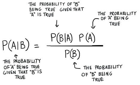
P(A|B) = P(B|A) \* P(A) / P(B)
Where:
- P(A|B) is the conditional probability of event A occurring given that event B has occurred.
- P(B|A) is the conditional probability of event B occurring given that event A has occurred.
- P(A) is the prior probability of event A occurring.
- P(B) is the prior probability of event B occurring.
This formula can be broken down into three components:
- The prior probability of event A, which represents our initial belief about the probability of event A occurring.
- The likelihood of event B given event A, which represents the probability of observing event B given that event A has occurred.
- The normalizing constant, which ensures that the resulting probability is between 0 and 1.
By understanding the components of Bayes’ formula, we can appreciate its power in updating probabilities based on new information. In the next section, we will explore how to apply Bayes’ formula in practice, including examples and illustrations to help readers understand the process.
How to Apply Bayes’ Formula: A Step-by-Step Guide
Now that we have a solid understanding of Bayes’ formula, let’s dive into a practical guide on how to apply it. This step-by-step guide will walk you through the process of using Bayes’ formula for conditional probability, including examples and illustrations to help you understand the process.
Step 1: Define the Problem
Identify the problem you want to solve using Bayes’ formula. This could be determining the probability of a disease given a positive test result, or the probability of a stock price increasing given a certain economic indicator.
Step 2: Identify the Variables
Identify the variables involved in the problem. In the case of Bayes’ formula, these are:
- P(A|B): the conditional probability of event A occurring given that event B has occurred.
- P(B|A): the conditional probability of event B occurring given that event A has occurred.
- P(A): the prior probability of event A occurring.
- P(B): the prior probability of event B occurring.
Step 3: Assign Probabilities
Assign probabilities to each of the variables identified in Step 2. These probabilities can be based on historical data, expert opinion, or other sources.
Step 4: Plug in the Values
Plug the assigned probabilities into Bayes’ formula:
P(A|B) = P(B|A) \* P(A) / P(B)
Step 5: Calculate the Result
Calculate the result of the formula, ensuring that the probability is between 0 and 1.
Example: Suppose we want to determine the probability of a person having a disease given that they have tested positive for it. We know that 90% of people with the disease test positive, and 10% of people without the disease test positive. We also know that 1% of the population has the disease.
Using Bayes’ formula, we can calculate the probability of a person having the disease given a positive test result:
P(Disease|Positive Test) = P(Positive Test|Disease) \* P(Disease) / P(Positive Test)
P(Disease|Positive Test) = 0.9 \* 0.01 / 0.1 = 0.81
Therefore, the probability of a person having the disease given a positive test result is 81%.
By following these steps and accurately calculating the probabilities, you can unlock the power of Bayes’ formula for conditional probability and make informed decisions in a variety of fields.
Real-World Applications of Bayes’ Formula: From Medicine to Finance
Bayes’ formula for conditional probability has far-reaching applications in various fields, including medicine, finance, and machine learning. In this section, we’ll explore some concrete examples to demonstrate the formula’s relevance and impact.
In Medicine:
Bayes’ formula is widely used in medical diagnosis to calculate the probability of a disease given a set of symptoms or test results. For instance, a doctor may use Bayes’ formula to determine the probability of a patient having a certain disease based on their symptoms, medical history, and test results. This helps doctors make informed decisions about treatment and further testing.
In Finance:
Bayes’ formula is used in finance to calculate the probability of a stock price increasing or decreasing based on historical data and market trends. This helps investors and analysts make informed decisions about investments and risk management.
In Machine Learning:
Bayes’ formula is used in machine learning to update the probability of a model’s parameters given new data. This is particularly useful in Bayesian neural networks, where the formula is used to update the weights and biases of the network based on new training data.
Other Applications:
Bayes’ formula has many other applications, including:
- Quality control: to calculate the probability of a defect given a set of quality control metrics.
- Marketing: to calculate the probability of a customer responding to a marketing campaign given their demographics and behavior.
- Insurance: to calculate the probability of a claim given a set of risk factors.
These examples illustrate the power of Bayes’ formula for conditional probability in real-world applications. By applying the formula, professionals in various fields can make informed decisions, update their knowledge, and improve their outcomes.
The bayes formula for conditional probability is a powerful tool that has far-reaching applications in many fields. By understanding how to apply the formula, professionals can unlock its potential and make a significant impact in their respective fields.
Common Misconceptions and Pitfalls: Avoiding Errors in Bayes’ Formula
When applying Bayes’ formula for conditional probability, it’s essential to avoid common mistakes and misconceptions that can lead to inaccurate results. In this section, we’ll discuss some of the most common pitfalls and provide tips on how to avoid them.
Incorrect Assumptions:
One of the most common mistakes is making incorrect assumptions about the prior probability or the likelihood function. This can lead to inaccurate calculations and misinterpretation of results. To avoid this, it’s essential to carefully define the problem and ensure that the assumptions are reasonable and well-supported.
Calculation Errors:
Calculation errors can occur when applying Bayes’ formula, especially when dealing with complex calculations. To avoid this, it’s essential to double-check calculations and ensure that the formula is applied correctly.
Ignoring Prior Knowledge:
Another common mistake is ignoring prior knowledge or expertise when applying Bayes’ formula. This can lead to inaccurate results and a failure to incorporate valuable insights. To avoid this, it’s essential to incorporate prior knowledge and expertise into the calculation.
Misinterpreting Results:
Misinterpreting the results of Bayes’ formula is another common pitfall. This can occur when the results are not properly understood or when they are over-interpreted. To avoid this, it’s essential to carefully interpret the results and ensure that they are properly understood.
Tips for Avoiding Pitfalls:
To avoid these common pitfalls, it’s essential to:
- Clearly define the problem and ensure that the assumptions are reasonable and well-supported.
- Double-check calculations and ensure that the formula is applied correctly.
- Incorporate prior knowledge and expertise into the calculation.
- Carefully interpret the results and ensure that they are properly understood.
By following these tips, professionals can avoid common mistakes and misconceptions when applying Bayes’ formula for conditional probability, ensuring accurate results and informed decision-making.
The bayes formula for conditional probability is a powerful tool, but it requires careful application to avoid errors and ensure accurate results. By understanding common pitfalls and taking steps to avoid them, professionals can unlock the full potential of Bayes’ formula and make informed decisions.
Bayes’ Formula vs. Frequentist Approach: Understanding the Difference
In the realm of statistics and probability, there are two primary approaches: Bayesian and frequentist. Bayes’ formula for conditional probability is a fundamental concept in Bayesian statistics, but it’s essential to understand how it differs from the frequentist approach. In this section, we’ll explore the strengths and weaknesses of each approach and explain when to use Bayes’ formula and when to opt for the frequentist approach.
Frequentist Approach:
The frequentist approach is based on the idea that probability is a long-run frequency of events. It focuses on the number of times an event occurs in a large number of trials. In this approach, probability is viewed as a property of the data, and statistical inference is based on the sample data.
Bayesian Approach:
The Bayesian approach, on the other hand, views probability as a degree of belief or uncertainty. It incorporates prior knowledge and expertise into the calculation, allowing for more flexible and nuanced modeling. Bayes’ formula for conditional probability is a cornerstone of Bayesian statistics, enabling the updating of probabilities based on new evidence.
Key Differences:
The primary differences between the Bayesian and frequentist approaches lie in their philosophical foundations and methodological approaches. The Bayesian approach is more flexible and adaptable, allowing for the incorporation of prior knowledge and expertise. The frequentist approach, while more traditional, is often limited by its reliance on sample data.
When to Use Bayes’ Formula:
Bayes’ formula is particularly useful in situations where:
- Prior knowledge or expertise is available and relevant.
- The problem involves conditional probability or updating probabilities based on new evidence.
- A more nuanced and flexible modeling approach is required.
When to Use the Frequentist Approach:
The frequentist approach is more suitable in situations where:
- The data is abundant and reliable.
- The problem involves estimating population parameters from sample data.
- A more traditional and widely accepted approach is required.
In conclusion, understanding the differences between Bayes’ formula and the frequentist approach is crucial for selecting the appropriate statistical methodology. By recognizing the strengths and weaknesses of each approach, professionals can make informed decisions and choose the most suitable method for their specific problem or application.
The bayes formula for conditional probability is a powerful tool in the Bayesian approach, offering a flexible and adaptable framework for modeling uncertainty. By understanding its differences with the frequentist approach, professionals can unlock the full potential of Bayes’ formula and make more informed decisions.
Advanced Topics in Bayes’ Formula: Prior Distributions and Hyperparameters
In the realm of Bayesian inference, prior distributions and hyperparameters play a crucial role in Bayes’ formula for conditional probability. These advanced topics enable a more nuanced and flexible approach to modeling uncertainty, allowing for more accurate predictions and informed decision-making.
Prior Distributions:
A prior distribution is a probability distribution that represents the initial beliefs or knowledge about a parameter before observing any data. In Bayes’ formula, the prior distribution is updated based on new evidence, resulting in a posterior distribution. The choice of prior distribution is critical, as it can significantly impact the results of Bayesian inference.
Common prior distributions include:
- Uniform distribution: A flat, uninformative prior that assigns equal probability to all possible values.
- Normal distribution: A continuous distribution that models symmetric, bell-shaped data.
- Beta distribution: A continuous distribution that models proportions or probabilities.
Hyperparameters:
Hyperparameters are parameters that govern the prior distribution. They are often fixed or set before observing the data and can significantly impact the results of Bayesian inference. Hyperparameters can be thought of as “parameters of parameters,” as they influence the shape and behavior of the prior distribution.
Examples of hyperparameters include:
- Variance or standard deviation: Controls the spread or dispersion of the prior distribution.
- Mean or location: Influences the central tendency of the prior distribution.
- Shape parameters: Affects the shape or skewness of the prior distribution.
Applications of Prior Distributions and Hyperparameters:
The combination of prior distributions and hyperparameters enables a more flexible and nuanced approach to Bayesian inference. This is particularly useful in:
- Machine learning: Prior distributions and hyperparameters can be used to model complex relationships and uncertainty in machine learning algorithms.
- Signal processing: Hyperparameters can be used to model signal noise and uncertainty in signal processing applications.
- Medical research: Prior distributions can be used to model the uncertainty associated with medical diagnoses or treatment outcomes.
In conclusion, prior distributions and hyperparameters are essential components of Bayes’ formula for conditional probability. By understanding their roles and applications, professionals can unlock the full potential of Bayesian inference and make more informed decisions in a wide range of fields.
The bayes formula for conditional probability is a powerful tool in Bayesian statistics, and mastering prior distributions and hyperparameters is crucial for accurate and reliable results. By incorporating these advanced topics into their workflow, professionals can take their Bayesian analysis to the next level.
Conclusion: Mastering Bayes’ Formula for Conditional Probability
In conclusion, Bayes’ formula for conditional probability is a powerful tool for making informed decisions in a wide range of fields. By understanding the concept of conditional probability, the mathematical breakdown of Bayes’ formula, and its various applications, professionals can unlock the full potential of Bayesian inference.
Throughout this guide, we have explored the importance of accurate calculations and interpretation, common misconceptions and pitfalls, and the differences between Bayes’ formula and the frequentist approach. We have also delved into advanced topics such as prior distributions and hyperparameters, highlighting their roles in Bayesian inference.
As we have seen, the bayes formula for conditional probability has far-reaching implications in fields such as medicine, finance, and machine learning. By mastering Bayes’ formula, professionals can make more accurate predictions, identify patterns, and drive informed decision-making.
It is essential to remember that Bayes’ formula is not a one-size-fits-all solution. Rather, it is a flexible and adaptable tool that can be tailored to specific problems and applications. By practicing and applying Bayes’ formula in their own work, professionals can develop a deeper understanding of conditional probability and unlock new insights and opportunities.
In the world of data analysis and decision-making, Bayes’ formula for conditional probability is an indispensable tool. By mastering this formula, professionals can stay ahead of the curve and drive success in their respective fields.

