The Importance of Skewness in Data Analysis
Skewness is a critical concept in data analysis and statistical modeling, referring to the asymmetry of a distribution around its mean. Positive skew and negative skew indicate the direction and magnitude of this asymmetry, with implications for data interpretation and decision-making. Understanding skewness is essential for accurately interpreting statistical measures such as mean, median, and mode, and for selecting appropriate models and techniques for data analysis.
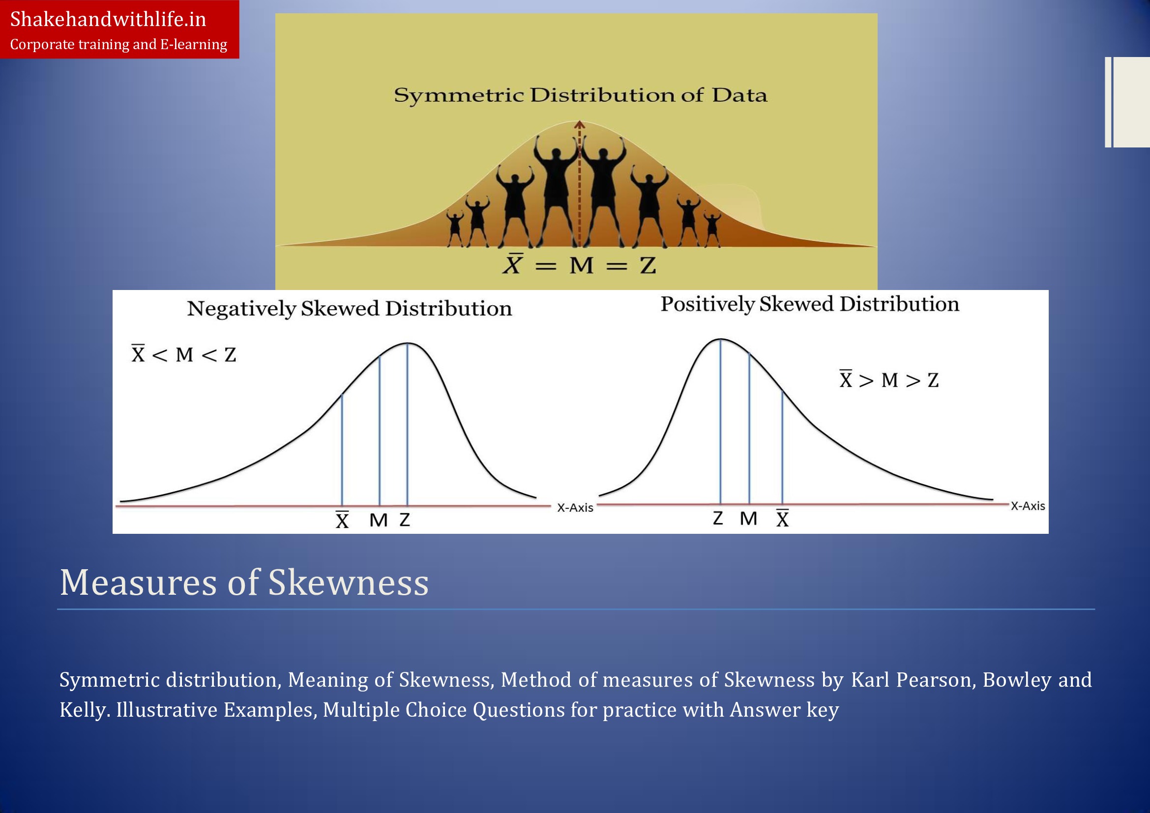
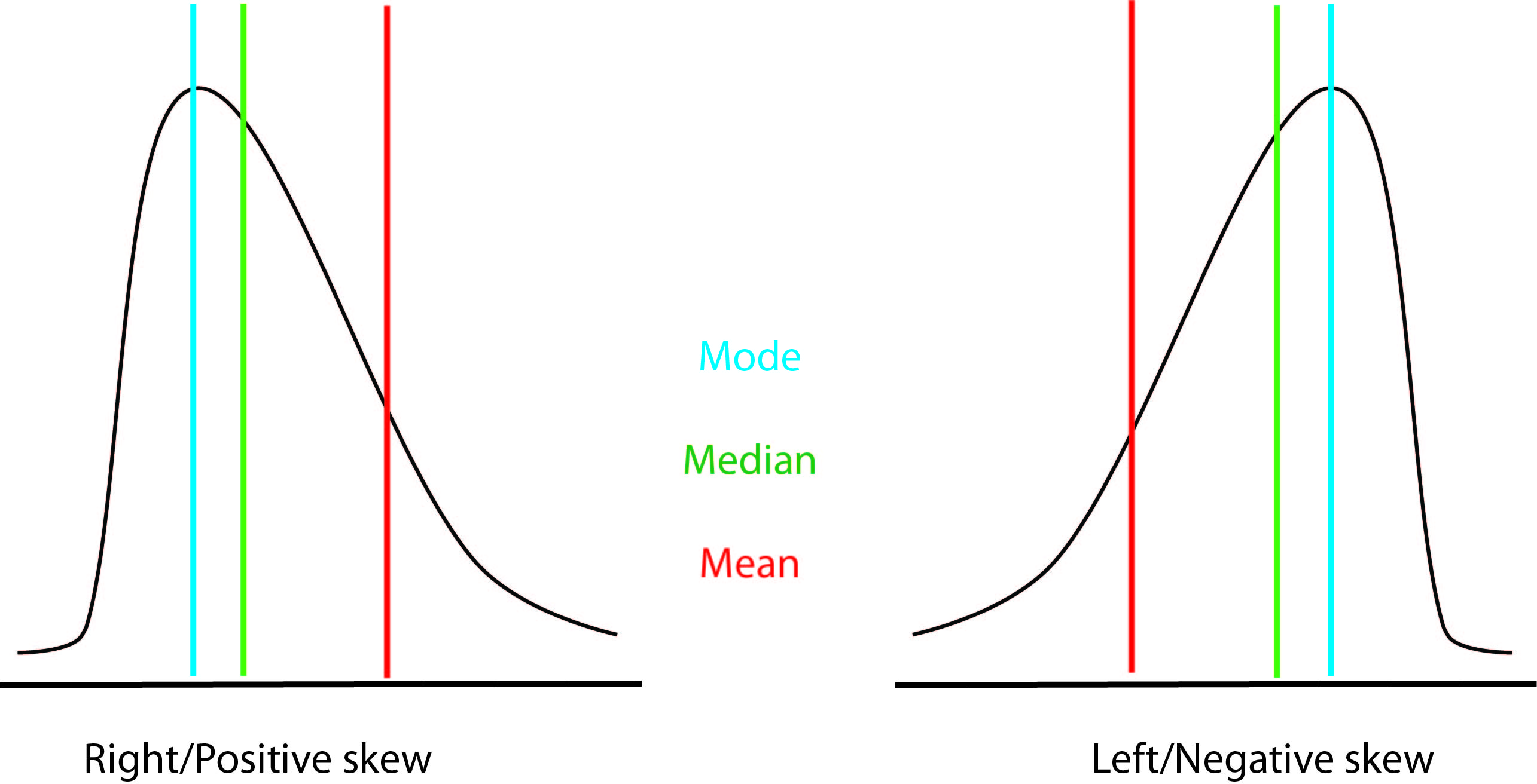
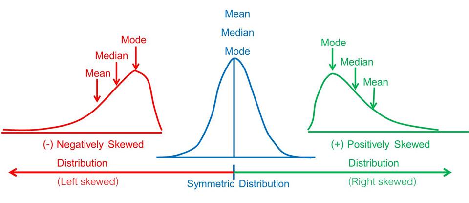
In a distribution with positive skew, the tail points to the right, indicating that the data values are concentrated on the left side of the distribution. This can result in a mean that is greater than the median, as the few extreme values on the right side of the distribution can significantly impact the mean. In contrast, negative skew indicates that the tail points to the left, with data values concentrated on the right side of the distribution. In this case, the mean may be lower than the median, as the extreme values on the left side of the distribution have less influence on the mean.
Ignoring skewness in data analysis can lead to inaccurate conclusions and misleading insights, as statistical measures and models may not adequately capture the underlying patterns and relationships in the data. For example, assuming a normal distribution when the data are skewed can result in underestimating variability and overestimating significance. Therefore, it is essential to identify and address skewness in data analysis, using techniques such as data transformation, outlier detection, and robust statistical methods.
Incorporating the concept of skewness in data analysis can provide valuable insights and improve decision-making in various fields, from finance and economics to healthcare and social sciences. By understanding the direction and magnitude of skewness, analysts and researchers can identify trends, patterns, and anomalies in the data, and develop effective strategies for data modeling, prediction, and optimization. Moreover, recognizing the limitations and assumptions of statistical methods and models can help ensure the validity and reliability of data analysis and avoid common pitfalls and misconceptions in skewness analysis.
Identifying Positive Skew: Characteristics and Examples
Positive skew, also known as right-skewed distribution, refers to a distribution where the tail points to the right, and the majority of the data points are concentrated on the left side of the distribution. The mean is greater than the median, and the mode is located on the left side of the distribution. Positive skew is often observed in data sets with extreme values or outliers on the right side of the distribution.
For example, in a data set of household incomes, a majority of the households may have incomes below $100,000, while a few households have incomes above $500,000. This results in a positively skewed distribution, where the mean is greater than the median, and the tail points to the right. Another example is in a data set of test scores, where a majority of the students score below 90, while a few students score above 95. This also results in a positively skewed distribution, where the mean is greater than the median, and the tail points to the right.
The shape of a positively skewed distribution is asymmetrical, with a longer right tail. The mean is influenced by the extreme values on the right side of the distribution, while the median is less affected. The mode is the most frequently occurring value in the distribution, which is located on the left side of the distribution. Positive skew can impact data interpretation and decision-making, as the mean may not accurately represent the central tendency of the data. Therefore, it is essential to consider skewness when analyzing data and making data-driven decisions.
Identifying Negative Skew: Characteristics and Examples
Negative skew, also known as left-skewed distribution, refers to a distribution where the tail points to the left, and the majority of the data points are concentrated on the right side of the distribution. The mean is less than the median, and the mode is located on the right side of the distribution. Negative skew is often observed in data sets with extreme values or outliers on the left side of the distribution.
For example, in a data set of rainfall amounts, a majority of the days may have rainfall below 10mm, while a few days have rainfall above 50mm. This results in a negatively skewed distribution, where the mean is less than the median, and the tail points to the left. Another example is in a data set of house prices, where a majority of the houses are priced below $500,000, while a few houses are priced above $1 million. This also results in a negatively skewed distribution, where the mean is less than the median, and the tail points to the left.
The shape of a negatively skewed distribution is asymmetrical, with a longer left tail. The mean is influenced by the extreme values on the left side of the distribution, while the median is less affected. The mode is the most frequently occurring value in the distribution, which is located on the right side of the distribution. Negative skew can impact data interpretation and decision-making, as the mean may not accurately represent the central tendency of the data. Therefore, it is essential to consider skewness when analyzing data and making data-driven decisions.
Measuring Skewness: Common Methods and Formulas
Skewness is a measure of the asymmetry of a distribution around its mean. There are several methods for measuring skewness, but the two most commonly used are the Pearson’s skewness coefficient and the Fisher-Pearson standardized skewness.
Pearson’s Skewness Coefficient
The Pearson’s skewness coefficient, also known as the Pearson’s moment coefficient of skewness, is a measure of the skewness of a distribution. It is calculated as the third standardized moment, which is the third moment of the distribution divided by the cube of the standard deviation. The formula for the Pearson’s skewness coefficient is:
Where is the third moment of the distribution, and is the cube of the standard deviation. A Pearson’s skewness coefficient of zero indicates a symmetrical distribution, while a positive value indicates a positively skewed distribution, and a negative value indicates a negatively skewed distribution.
Fisher-Pearson Standardized Skewness
The Fisher-Pearson standardized skewness is another measure of skewness that is commonly used. It is calculated as the Pearson’s skewness coefficient divided by the standard error of the skewness. The formula for the Fisher-Pearson standardized skewness is:
Where is the Pearson’s skewness coefficient, and is the standard error of the skewness. A Fisher-Pearson standardized skewness of zero indicates a symmetrical distribution, while a positive value indicates a positively skewed distribution, and a negative value indicates a negatively skewed distribution.
Both the Pearson’s skewness coefficient and the Fisher-Pearson standardized skewness are useful measures of skewness, and the choice of which to use depends on the specific needs of the analysis. The Pearson’s skewness coefficient is more sensitive to extreme values, while the Fisher-Pearson standardized skewness is more robust to outliers. It is important to note that both measures of skewness assume a normal distribution, and may not be accurate for non-normal distributions.
How to Interpret Skewness: Implications for Data Analysis
Skewness is an essential concept in statistical analysis, as it can significantly impact data interpretation and decision-making. Positive and negative skew can affect the mean, median, and mode of a distribution, and understanding these relationships is crucial for accurate data analysis.
Mean, Median, and Mode
The mean, median, and mode are three common measures of central tendency used in statistical analysis. The mean is the average of all data points, the median is the middle value when the data is sorted in ascending order, and the mode is the most frequently occurring value in the data set. In a symmetrical distribution, the mean, median, and mode are equal, but in a skewed distribution, these measures can differ.
Positive Skew
In a positively skewed distribution, the tail points to the right, and the majority of the data points are concentrated on the left side of the distribution. The mean is greater than the median, and the mode is located on the left side of the distribution. Positive skew can indicate the presence of outliers or extreme values on the right side of the distribution, which can significantly impact the mean.
Negative Skew
In a negatively skewed distribution, the tail points to the left, and the majority of the data points are concentrated on the right side of the distribution. The mean is less than the median, and the mode is located on the right side of the distribution. Negative skew can also indicate the presence of outliers or extreme values, but on the left side of the distribution.
Considering Skewness in Data-Driven Decisions
When analyzing skewed data, it is essential to consider the implications of skewness on the measures of central tendency. In a positively skewed distribution, the mean may not accurately represent the central tendency of the data, and the median may be a more appropriate measure. In a negatively skewed distribution, the opposite is true. Additionally, skewness can impact the variability of the data, as measured by the standard deviation. Therefore, it is crucial to consider skewness when making data-driven decisions.
Tips for Accurate Data Interpretation
To ensure accurate data interpretation, it is essential to:
- Identify skewness in the data distribution
- Understand the impact of skewness on the measures of central tendency
- Consider the implications of skewness on data interpretation and decision-making
- Use appropriate statistical methods for skewed data, such as transformations or non-parametric tests
- Avoid making assumptions about the data, such as assuming normality or equal variances
By following these tips, analysts can ensure accurate data interpretation and make informed, data-driven decisions.
Transforming Skewed Data: Techniques and Best Practices
Skewness can significantly impact data analysis and interpretation, and transforming skewed data can help to mitigate these effects. There are several techniques for transforming skewed data, each with its benefits and limitations. In this section, we will discuss two common methods: logarithmic and square root transformations.
Logarithmic Transformation
A logarithmic transformation is a non-linear transformation that can be used to reduce positive skew in a data set. This method involves taking the natural logarithm of each data point, which can help to normalize the distribution and reduce the impact of outliers. The logarithmic transformation is most effective for data sets with a large range of values and a long right tail. However, this method is not appropriate for data sets with zero or negative values, as the logarithm of zero is undefined.
Square Root Transformation
A square root transformation is another non-linear transformation that can be used to reduce positive skew in a data set. This method involves taking the square root of each data point, which can help to normalize the distribution and reduce the impact of outliers. The square root transformation is most effective for data sets with a moderate range of values and a shorter right tail. However, this method can be less effective than the logarithmic transformation for data sets with a large range of values.
Benefits and Limitations
Both the logarithmic and square root transformations can be effective for reducing positive skew in a data set. However, there are some benefits and limitations to consider:
- Benefits:
- Reduces positive skew and normalizes the distribution
- Mitigates the impact of outliers
- Improves the accuracy of statistical analysis and interpretation
- Limitations:
- May not be appropriate for data sets with zero or negative values
- May require additional data manipulation and analysis
- May not completely eliminate skewness in some cases
Examples of Application
Let’s consider an example of a data set with positive skew:
- Data set: Income (in dollars) of 100 individuals:
- 500, 1000, 1500, 2000, 2500, 3000, 3500, 4000, 4500, 5000, 5500, 6000, 6500, 7000, 7500, 8000, 8500, 9000, 9500, 10000, 10500, 11000, 11500, 12000, 12500, 13000, 13500, 14000, 14500, 15000, 15500, 16000, 16500, 17000, 17500, 18000, 18500, 19000, 19500, 20000, 25000, 30000, 50000
We can apply a logarithmic transformation to this data set to reduce the positive skew:
- Transformed data set: ln(Income) (in dollars):
- 6.21, 6.91, 7.32, 7.60, 7.92, 8.20, 8.45, 8.67, 8.89, 9.09, 9.27, 9.44, 9.59, 9.74, 9.87, 9.99, 10.10, 10.21, 10.31, 10.40, 10.48, 10.56, 10.64, 10.71, 10.78, 10.85, 10.91, 10.97, 11.03, 11.08, 11.13, 11.18, 11.23, 11.27, 11.32, 11.36, 11.40, 11.44, 11.49, 11.57, 11.71, 12.20
We can see that the transformed data set has a more normal distribution, with a reduced impact of outliers.
Conclusion
Transforming skewed data can help to mitigate the impact of skewness on data analysis and interpretation. Logarithmic and square root transformations are two common methods for transforming skewed data, each with its benefits and limitations. By understanding these techniques and their applications, analysts can ensure accurate data interpretation and make informed, data-driven decisions.
Software Tools for Skewness Analysis: A Comparison
Analyzing skewness in data can be done using various software tools, each with its strengths and weaknesses. In this section, we will compare three popular software tools for skewness analysis: Excel, R, and Python.
Excel
Microsoft Excel is a widely used spreadsheet software that includes various statistical functions for data analysis. Excel can calculate skewness using the built-in function SKEW(). However, Excel does not provide a direct function for measuring skewness with the Fisher-Pearson standardized method. Excel is user-friendly and accessible, making it a good option for beginners or those who prefer a graphical user interface.
R
R is a programming language and software environment for statistical computing and graphics. R has various packages for data analysis, including the moments package, which provides functions for calculating skewness using both the Pearson’s and Fisher-Pearson standardized methods. R is a powerful tool for data analysis, but it has a steeper learning curve compared to Excel. R is also open-source, making it a cost-effective option for data analysis.
Python
Python is a high-level, general-purpose programming language with various libraries for data analysis, including numpy and scipy. These libraries provide functions for calculating skewness using both the Pearson’s and Fisher-Pearson standardized methods. Python is a versatile tool for data analysis, but it has a steeper learning curve compared to Excel and R. Python is also open-source, making it a cost-effective option for data analysis.
Comparison
Here is a comparison of the three software tools for skewness analysis:
| Software Tool | Pearson’s Skewness | Fisher-Pearson Standardized Skewness | User-Friendliness | Cost |
|---|---|---|---|---|
| Excel | Yes | No | High | Paid |
| R | Yes | Yes | Medium | Open-source |
| Python | Yes | Yes | Medium | Open-source |
Excel is a user-friendly option for calculating skewness using the Pearson’s method, but it does not provide a direct function for the Fisher-Pearson standardized method. R and Python are both powerful tools for data analysis and provide functions for calculating skewness using both methods. R and Python have a steeper learning curve compared to Excel, but they are open-source and cost-effective options for data analysis.
Conclusion
Understanding skewness in data is essential for accurate data interpretation and decision-making. Various software tools can be used for skewness analysis, each with its strengths and weaknesses. Excel is a user-friendly option for calculating skewness using the Pearson’s method, while R and Python are powerful tools that provide functions for calculating skewness using both the Pearson’s and Fisher-Pearson standardized methods. By choosing the appropriate software tool and technique, analysts can ensure accurate data interpretation and make informed, data-driven decisions.
Common Pitfalls and Misconceptions in Skewness Analysis
Analyzing skewness in data can be a complex process, and there are several common pitfalls and misconceptions that analysts should be aware of. Here are some tips for avoiding these mistakes and ensuring accurate data interpretation:
- Assuming that skewness is always a problem: Skewness is a natural occurrence in many data sets and is not necessarily a problem. It is essential to interpret skewness in the context of the data and the research question. In some cases, skewness may be inconsequential or even beneficial to the analysis.
- Neglecting the impact of outliers: Outliers can have a significant impact on skewness, and it is essential to identify and address outliers before analyzing skewness. Outliers can be caused by errors in data collection or entry, or they may represent extreme but valid observations. In either case, outliers should be carefully examined and addressed before analyzing skewness.
- Using the wrong measure of skewness: There are several methods for measuring skewness, and it is essential to choose the appropriate method for the data and the research question. The Pearson’s skewness coefficient and the Fisher-Pearson standardized skewness are two commonly used methods, but there are others that may be more appropriate in certain situations.
- Ignoring the impact of sample size: Sample size can have a significant impact on skewness, and it is essential to consider the sample size when interpreting skewness. In general, larger sample sizes are more likely to produce normally distributed data, while smaller sample sizes are more likely to produce skewed data. It is essential to interpret skewness in the context of the sample size and the research question.
- Failing to transform skewed data: In some cases, transforming skewed data can help to normalize the distribution and improve the accuracy of statistical analysis. Logarithmic or square root transformations are two common methods for transforming skewed data, but there are others that may be more appropriate in certain situations. It is essential to carefully consider the benefits and limitations of each method before transforming skewed data.
Conclusion
Understanding skewness in data is essential for accurate data interpretation and decision-making. Analyzing skewness can help to identify outliers, normalize data distributions, and improve the accuracy of statistical analysis. However, there are several common pitfalls and misconceptions that analysts should be aware of when analyzing skewness. By avoiding these mistakes and ensuring accurate data interpretation, analysts can make informed, data-driven decisions that are based on a thorough understanding of the data.


