Unlocking the Power of Stochastic Processes in Finance
In the field of financial modeling, geometric Brownian motion has emerged as a powerful tool for simulating and analyzing complex financial systems. This stochastic process has been widely adopted in finance due to its ability to accurately model stock prices and portfolio returns. By harnessing the power of geometric Brownian motion in R, financial professionals can gain valuable insights into market trends, optimize portfolio performance, and make informed investment decisions. The ability to simulate stock prices and portfolio returns using geometric Brownian motion in R has made it an indispensable tool in finance, with applications ranging from option pricing to risk management and portfolio optimization.

Click Image to Find Quantum Products

Understanding the Math Behind Geometric Brownian Motion
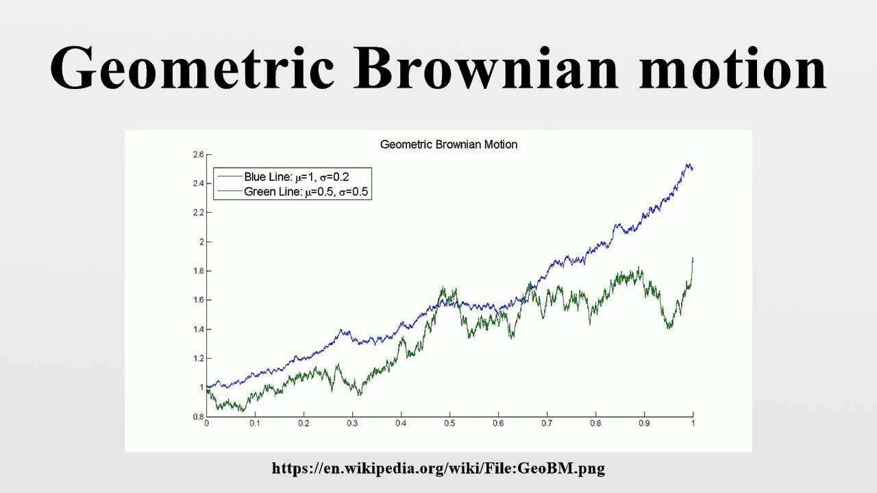
Geometric Brownian motion is a stochastic process that is widely used in finance to model stock prices and portfolio returns. Mathematically, it is formulated as a stochastic differential equation (SDE), which describes the evolution of a stock price over time. The SDE is typically denoted as dS(t) = μS(t)dt + σS(t)dW(t), where S(t) is the stock price at time t, μ is the drift parameter, σ is the volatility parameter, and W(t) is a Wiener process. The drift parameter represents the expected rate of return, while the volatility parameter represents the uncertainty or risk associated with the stock price. In the context of geometric Brownian motion in R, these parameters are crucial in determining the behavior of the simulated stock prices and portfolio returns.

How to Implement Geometric Brownian Motion in R
To implement geometric Brownian motion in R, several packages and functions can be utilized. One popular package is the sde package, which provides a range of functions for simulating stochastic differential equations. Specifically, the sde.sim function can be used to simulate geometric Brownian motion. The function requires input parameters such as the drift and volatility coefficients, as well as the time interval and number of simulations. For example, the following code can be used to simulate a geometric Brownian motion with a drift of 0.05 and volatility of 0.2: sde.sim(model = "GBM", drift = 0.05, sigma = 0.2, N = 1000, T = 1). This code will generate 1000 simulations of the geometric Brownian motion over a time period of 1 year. Additionally, the plot function can be used to visualize the results, providing a graphical representation of the simulated stock prices. By leveraging these packages and functions, users can easily implement geometric Brownian motion in R and apply it to a range of financial modeling tasks, including option pricing and risk management.

Simulating Stock Prices with Geometric Brownian Motion in R
One of the primary applications of geometric Brownian motion in R is simulating stock prices. By using the sde package and the sde.sim function, users can generate multiple simulations of stock prices over a specified time period. For example, the following code can be used to simulate the stock price of a company with a drift of 0.05 and volatility of 0.2 over a period of 1 year: sde.sim(model = "GBM", drift = 0.05, sigma = 0.2, N = 1000, T = 1). This code will generate 1000 simulations of the stock price, providing a range of possible outcomes. To visualize the results, the plot function can be used to create a graph of the simulated stock prices. This can be useful for identifying trends and patterns in the data, as well as for comparing the results of different simulations. Additionally, the simulated stock prices can be used as input for other financial models, such as option pricing models or risk management models. By leveraging geometric Brownian motion in R, users can generate realistic and accurate simulations of stock prices, which can be used to inform investment decisions and improve financial modeling outcomes.
In addition to simulating stock prices, geometric Brownian motion in R can also be used to simulate portfolio returns. By simulating the returns of multiple assets, users can analyze the performance of different portfolios and identify the most effective investment strategies. This can be particularly useful for investors and financial analysts, who need to make informed decisions about asset allocation and risk management. By using geometric Brownian motion in R, users can generate realistic and accurate simulations of portfolio returns, which can be used to inform investment decisions and improve financial outcomes.
Applications of Geometric Brownian Motion in Finance
Geometric Brownian motion in R has a wide range of applications in finance, including option pricing, risk management, and portfolio optimization. One of the most significant applications is in option pricing, where geometric Brownian motion is used to model the underlying asset price. This allows for the calculation of option prices and Greeks, such as delta and gamma, which are essential for risk management and hedging strategies. Additionally, geometric Brownian motion can be used to simulate the behavior of complex financial instruments, such as exotic options and structured products.
In risk management, geometric Brownian motion in R can be used to simulate potential losses and gains, allowing for the calculation of Value-at-Risk (VaR) and Expected Shortfall (ES). This enables financial institutions to better manage their risk exposure and make informed decisions about capital allocation. Furthermore, geometric Brownian motion can be used to optimize portfolio performance by identifying the most efficient asset allocation and minimizing risk.
Another application of geometric Brownian motion in R is in credit risk modeling, where it can be used to simulate the behavior of credit ratings and default probabilities. This allows for the calculation of credit losses and the optimization of credit portfolios. Moreover, geometric Brownian motion can be used in asset liability management, where it can be used to simulate the behavior of assets and liabilities, allowing for the optimization of asset allocation and liability hedging strategies.
In addition to these applications, geometric Brownian motion in R can also be used in other areas of finance, such as derivatives pricing, risk analysis, and portfolio optimization. Its ability to simulate complex financial systems and provide accurate predictions makes it an essential tool for financial modeling and analysis. By leveraging geometric Brownian motion in R, financial professionals can gain a deeper understanding of financial markets and make more informed investment decisions.

Common Pitfalls and Challenges in Implementing Geometric Brownian Motion
While geometric Brownian motion in R is a powerful tool for financial modeling, there are several common pitfalls and challenges that users may encounter when implementing it. One of the most significant challenges is parameter estimation, where the drift and volatility parameters must be accurately estimated to ensure reliable results. This can be a complex task, especially when dealing with large datasets or noisy data.
Another common pitfall is model validation, where the geometric Brownian motion model must be validated against historical data to ensure that it accurately captures the underlying dynamics of the financial system. This can be a time-consuming process, requiring careful analysis and testing of the model.
In addition, users may encounter issues with numerical instability, where the simulation results may be sensitive to the choice of time step or numerical method. This can lead to inaccurate or unreliable results, and requires careful attention to the numerical implementation of the model.
Furthermore, geometric Brownian motion in R may not always be suitable for modeling complex financial systems, where non-linear or non-Gaussian dynamics may be present. In such cases, more advanced models, such as stochastic volatility models or jump-diffusion models, may be required.
To overcome these challenges, users must have a deep understanding of the mathematical formulation of geometric Brownian motion, as well as the numerical implementation in R. Additionally, careful attention must be paid to parameter estimation, model validation, and numerical stability to ensure reliable and accurate results.
By being aware of these common pitfalls and challenges, users can take steps to mitigate them and ensure that their implementation of geometric Brownian motion in R is successful. This includes using robust parameter estimation methods, carefully validating the model, and carefully implementing the numerical simulation.
Advanced Topics in Geometric Brownian Motion: Multivariate and Non-Stationary Models
In addition to the basic geometric Brownian motion model, there are several advanced topics that can be explored to further enhance the accuracy and flexibility of financial modeling. One such topic is multivariate geometric Brownian motion, which allows for the simulation of multiple correlated assets or risk factors. This is particularly useful in portfolio optimization and risk management, where the relationships between different assets must be taken into account.
Another advanced topic is non-stationary geometric Brownian motion, which allows for the simulation of assets with time-varying drift and volatility parameters. This is particularly useful in modeling assets with changing market conditions or regime shifts. Non-stationary geometric Brownian motion can be implemented in R using techniques such as regime-switching models or time-varying parameter estimation.
These advanced topics in geometric Brownian motion in R can be used to model complex financial systems and provide more accurate and realistic simulations. For example, multivariate geometric Brownian motion can be used to model the behavior of a portfolio of stocks, bonds, and commodities, while non-stationary geometric Brownian motion can be used to model the behavior of an asset with changing market conditions.
In addition, these advanced topics can be used to develop more sophisticated financial models, such as stochastic volatility models or jump-diffusion models. These models can be used to capture more complex dynamics and provide more accurate predictions of financial outcomes.
By exploring these advanced topics in geometric Brownian motion in R, users can unlock the full potential of this powerful tool and develop more sophisticated and accurate financial models. This can lead to better investment decisions, more effective risk management, and improved portfolio performance.
Overall, the advanced topics in geometric Brownian motion in R provide a powerful framework for modeling complex financial systems and simulating realistic scenarios. By mastering these topics, users can take their financial modeling to the next level and achieve greater success in the world of finance.
Conclusion: Unlocking the Full Potential of Geometric Brownian Motion in R
In conclusion, geometric Brownian motion in R is a powerful tool for financial modeling, offering a flexible and realistic way to simulate stock prices and portfolio returns. By understanding the mathematical formulation of geometric Brownian motion and implementing it in R, users can unlock the full potential of this stochastic process and gain valuable insights into financial markets.
Throughout this article, we have explored the significance of geometric Brownian motion in financial modeling, delved into the mathematical formulation, and provided a step-by-step guide on how to implement it in R. We have also demonstrated how to simulate stock prices and discussed the various applications of geometric Brownian motion in finance.
In addition, we have highlighted common pitfalls and challenges that may arise when implementing geometric Brownian motion in R, and explored advanced topics such as multivariate and non-stationary models. By mastering these concepts, users can develop more sophisticated and accurate financial models, leading to better investment decisions and improved portfolio performance.
Geometric Brownian motion in R is a powerful tool that can be used to unlock the full potential of financial modeling. By leveraging the flexibility and realism of this stochastic process, users can gain a competitive edge in the world of finance and achieve greater success.
Whether you are a financial analyst, portfolio manager, or researcher, geometric Brownian motion in R is an essential tool to have in your toolkit. By mastering this powerful tool, you can unlock new insights, improve your financial models, and achieve greater success in the world of finance.
